1 Learning from Data
1.1 Cause-Effect Relationships
Why do people like to collect (nowadays, big) data? Typically, the goal is to find “relationships” between different “variables”: What fertilizer combination makes my plants grow tall? What medication reduces headache most? Is a new vaccine effective enough?
From a more abstract point of view, we are in the situation where we have a “system” or a “process” (e.g., a plant) with many input variables (so-called predictors) and an output (so-called response), see also Montgomery (2019). In the previous example the ingredients of the fertilizer are the inputs, and the output could be the biomass of a plant.
Ideally, we would like to find cause-effect relationships, meaning that when we actively change one of the inputs, i.e., we make an intervention on the system, this will cause the output to change. If we can just observe a system under different settings (so-called observational studies or observational data), it is much harder to make a statement about causal effects, as can be seen in the following examples:
Is the seatbelt sign on an airplane causing a plane to shake? If we could switch it on ourselves, would the plane start shaking? See The Family Circus comic strip (Keane 1998): “I wish they didn’t turn on that seatbelt sign so much! Every time they do, it gets bumpy.”
Are ice cream sales causing people to drown? If we would stop selling ice cream, would drowning decrease, or even stop?
With observational data, we can typically just make a statement about an association between two variables. One potential danger is the existence of confounding variables or confounders. A confounder is a common cause for two variables. In the previous examples we had the following situations:
Turbulent weather simultaneously makes the pilot switch on the seatbelt sign and the plane shake. What we observe is an association between the appearance of the seatbelt sign and a shaking plane. The seatbelt sign is not a cause of the shaking plane.
Hot weather makes people want to go swimming and at the same time is beneficial for ice cream sales. What we observe is an association between ice cream sales and the number of drowning incidents. Ice cream sales is not a cause of the number of drowning incidents.
A more classical example was the question whether smoking causes lung cancer or maybe “bad genes” make people smoke and develop lung cancer at the same time (Stolley 1991). More examples of spurious associations can be found on http://www.tylervigen.com/spurious-correlations.
To find out cause-effect relationships, we should ideally be able to make an intervention on a system ourselves. If we would occasionally switch on the seatbelt sign, ignoring the weather conditions, we would see that the plane will typically not start shaking. This is what we do in experimental studies. We actively change the inputs of the system, i.e., we make an intervention, and we observe what happens with the output. It is like reverse engineering the system to find out how it works. This is also how little kids or babies discover the world: “If I push this button then …”.
Remark: It is also possible to make a statement about causal effects using observational data. To do so, we would need to know the underlying “causal diagram”, typically unknown in practice, where direct causal effects are visualized by arrows. A set of rules (see for example Pearl and Mackenzie 2018) would then tell us what variables we have to consider in our analysis (“conditioning”). In the seatbelt sign example, if we also consider weather conditions, we would see that there is no causal effect from the seatbelt sign on the movements of the plane. The corresponding causal diagram would look like the one in Figure 1.1.
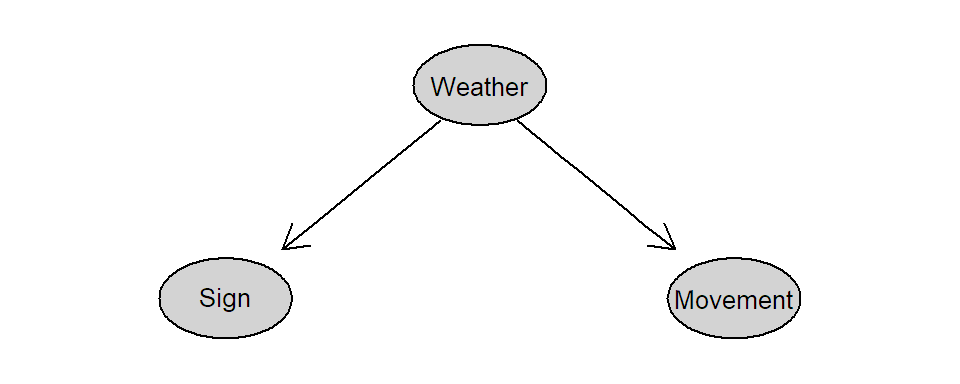
FIGURE 1.1: Causal diagram for the seatbelt sign example.
A more complicated example is illustrated in Figure 1.2. If we are interested in the total causal effect of “In” on “Out” using observational data, we would need to believe that this causal diagram is really representing the truth (in particular, we did not forget any important variables) and we have to derive the correct set of variables to condition on (here, only “D”). On the other hand, if we can do an experiment, we simply make an intervention on variable “In” and see what happens with the output “Out,” we do not have to know the underlying causal diagram.
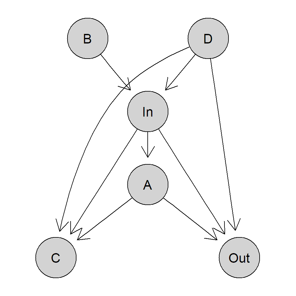
FIGURE 1.2: More general causal diagram.
1.2 Experimental Studies
In this section, we closely follow Chapter 1 of Oehlert (2000) to give you an idea of the main ingredients of an experimental study.
Before designing an experimental study, we must have a focused and precise research question that we want to answer with experimental data, e.g., “how does fertilizer \(A\) compare to fertilizer \(B\) with respect to biomass of plants after 10 weeks?”. Quite often, people collect large amounts of data and afterward think, “let’s see whether we find some interesting patterns in our data!”. Such an approach is permissible in order to create some research question. However, we focus on the part where we want to confirm a certain specific conjecture. We have to make sure that it is actually testable, i.e., that we can do the appropriate interventions and that we can measure the right response (see Section 1.2.4).
An experimental study consists of the following ingredients:
The different interventions which we perform on the system: the different treatments, e.g., different fertilizer combinations that we are interested in, but also other predictors (inputs) of the system (see Section 1.2.1).
Experimental units: the actual objects on which we apply the treatments, e.g., plots of land, patients, fish tanks, etc. (see Section 1.2.3).
A method that assigns experimental units to treatments, typically randomization or restricted versions thereof (see Section 1.2.2).
Response(s): the output that we measure, e.g., biomass of plants (see Section 1.2.4).
In addition, when designing an experimental study, the analysis of the resulting data should already be considered. For example, we need an idea of the experimental error (see Section 1.2.5); otherwise, we cannot do any statistical inference. It is always a good idea to try to analyze some simulated data before performing the experiment, as this can potentially already reveal some serious flaws of the design.
1.2.1 Predictors or Treatments
We distinguish between the following types of predictors (inputs of the system):
Predictors that are of primary interest and that can (ideally) be varied according to our “wishes”: the conditions we want to compare, or the treatments, e.g., fertilizer type.
Predictors that are systematically recorded such that potential effects can later be eliminated in our calculations (“controlling for …”), e.g., weather conditions. In this context, we also call them covariates.
Predictors that can be kept constant and whose effects are therefore eliminated, e.g., always using the same measurement device.
Predictors that we can neither record nor keep constant, e.g., some special soil properties that we cannot measure.
1.2.2 Randomization
Randomization, i.e., the random allocation of experimental units to the different treatments, ensures that the only systematic difference between the different treatment groups is the treatment: No matter what special properties the experimental units have, we have a similar mix in each group. This protects us from confounders and is the reason why a properly randomized experiment allows us to make a statement about a cause-effect relationship between treatment and response.
The importance of randomization is also nicely summarized in the following quote:
“Randomization generally costs little in time and trouble, but it can save us from disaster.” (Oehlert 2000)
We can and should also randomize other aspects like the sequence in which experimental units are measured. This protects us from time being a confounder.
Quite often, we already know that some experimental units are more alike than others before doing the experiment. Think for example of different locations for an agricultural experiment. Typically, we then do a randomization “within” homogeneous blocks (here, at each location). This restricted version of randomization is called blocking. A block is a subset of experimental units that is more homogeneous than the entire set. Blocking typically increases precision of an experiment, see Chapter 5. The rule to remember is:
“Block what you can; randomize what you cannot.” (George E. P. Box, Hunter, and Hunter 1978)
1.2.3 Experimental and Measurement Units
An experimental unit is defined as the object on which we apply the treatments by randomization. The general rule is (Oehlert 2000): “An experimental unit should be able to receive any treatment independently of the other units”. On the other hand, a measurement unit is the object on which the response is being measured. There are many situations where experimental units and measurement units are not the same. This can cause severe consequences on the analysis if not treated appropriately.
For example, if we randomize different food supplies to fish tanks (containing multiple fish), the experimental unit is given by a fish tank and not an individual fish. However, a measurement unit will be given by an individual fish, e.g., we could take as response the body weight of a fish after 5 weeks. Typically, we aggregate the values of the measurement units such that we get one value per experimental unit, e.g., take the average body weight per fish tank. These values will typically be the basis for the statistical analysis later on.
There are also situations where there are different “sizes” (large and small) of experimental units within the same experiment, see Chapter 7.
As we want our results to have broad validity, the experimental units should ideally be a random sample from the population of interest. If the experimental units do not represent the population well, drawing conclusions from the experimental results to the population will be challenging. In this regard, internal validity means that the study was set up and performed correctly with the experimental units at hand, e.g., by using randomization, blinding as mentioned below, etc. Hence, the conclusions that we draw are valid for the “study population”. On the other hand, external validity means that the conclusions can be transferred to a more general population. For example, if we properly run a psychological study with volunteers, we have internal validity. However, we do not necessarily have external validity if the volunteers do not represent the general population well (because they are not a random sample).
1.2.4 Response
The response, or the output of the process, should be chosen such that it reflects useful information about the process under study, e.g., body weight after some diet treatment or biomass when comparing different fertilizers. It is your responsibility that the response is a reasonable quantity to study your research hypothesis. There are situations where the response is not directly measurable. An example is HIV progression. In cases like this, we need a so-called surrogate response. For HIV, this could be CD4-cell counts. These cells are being attacked by HIV and the number gives you an idea of the health status of the immune system.
1.2.5 Experimental Error
Consider the following hypothetical example: We make an experiment using two plants. One gets fertilizer \(A\) and the other one \(B\). After 4 weeks, we observe that the plant receiving fertilizer \(A\) has twice the biomass of the plant receiving fertilizer \(B\). Can we conclude that fertilizer \(A\) is causing larger biomass? Unfortunately, we cannot say so in this situation, even if we randomized the two fertilizers to the two plants. The experiment does not give us any information whether the difference that we observe is larger than the natural variation from plant to plant getting the same fertilizer. It could very well be the case that there is no difference between the two fertilizers, meaning that the difference that we observe is just natural variation from plant to plant. From a technical point of view, this is like trying to do a two-sample \(t\)-test with only one observation in each group.
In other words, no two experimental units are perfectly identical. Hence, it is completely natural that we will measure slightly different values for the response, even if they get the same treatment. We should design our experiment such that we get an idea of this so-called experimental error. Here, this means we would need multiple plants (replicates) receiving the same treatment. If the difference between the treatments is much larger than the experimental error, we can conclude that there is a treatment effect caused by the fertilizer. You’ve learned analyzing such data with a two-sample \(t\)-test, which would not work with only one observation in each treatment group, see above.
A “true” replicate should be given by another independent experimental unit. If we would measure the biomass of the original two plants 10 times each, we would also have multiple measurements per treatment group. However, the error that we observe is simply the measurement error of our measurement device. Hence, we still have no clue about the experimental error. We would call them pseudoreplicates. From a technical point of view, we could do a two-sample \(t\)-test in this situation. However, we could just conclude that these two specific plants are different for whatever reason. This is not what you typically want to do.
1.2.6 More Terminology
Blinding means that those who measure or assess the response do not know which treatment is given to which experimental unit. With humans it is common to use double-blinding where in addition the patients do not know the assignment either. Blinding protects us from (unintentional) bias due to expectations.
A control treatment is typically a standard treatment with which we want to compare. It can also be no treatment at all. You should always ask yourself, “How does it compare to no treatment or the standard treatment?”. For example, a physiotherapist claims that a new therapy after surgery reduces pain by about 30%. However, patients without any therapy after surgery might have a reduction of 50%!
1.2.7 A Few Examples
What’s wrong with the following examples?
Mike is interested in the difference between two teaching techniques. He randomly selects 10 Harvard lecturers that apply technique \(A\) and 10 MIT lecturers that apply technique \(B\). Each lecturer reports the average grade of his class.
Linda has two cages of mice. Mice in cage 1 get a special food supply, while mice in cage 2 get ordinary food (control treatment).
Melanie offers a new exam preparation course. She claims that, on average, only 20% of her students fail the exam.