6 Random and Mixed Effects Models
In this chapter we use a new philosophy. Up to now, treatment effects (the \(\alpha_i\)’s) were fixed, unknown quantities that we tried to estimate. This means we were making a statement about a specific, fixed set of treatments (e.g., some specific fertilizers or different vaccine types). Such models are also called fixed effects models.
6.1 Random Effects Models
6.1.1 One-Way ANOVA
Now we use another point of view: We consider situations where treatments are random samples from a large population of treatments. This might seem quite special at first sight, but it is actually very natural in many situations. Think for example of investigating employee performance of those who were randomly selected. Another example could be machines that were randomly sampled from a large population of machines. Typically, we are interested in making a statement about some properties of the whole population and not of the observed individuals (here, employees or machines).
Going further with the machine example: Assume that every machine produces some samples whose quality we assess. We denote the observed quality of the \(j\)th sample on the \(i\)th machine with \(y_{ij}\). We can model such data with the model \[\begin{equation} Y_{ij} = \mu + \alpha_i + \epsilon_{ij}, \tag{6.1} \end{equation}\] where \(\alpha_i\) is the effect of the \(i\)th machine. As the machines were drawn randomly from a large population, we assume \[ \alpha_i \; \textrm{i.i.d.} \sim N(0, \sigma_{\alpha}^2). \] We call \(\alpha_i\) a random effect. Hence, (6.1) is a so-called random effects model. For the error term we have the usual assumption \(\epsilon_{ij}\) i.i.d. \(\sim N(0, \sigma^2)\). In addition, we assume that \(\alpha_i\) and \(\epsilon_{ij}\) are independent. This looks very similar to the old fixed effects model (2.4) at first sight. However, note that the \(\alpha_i\)’s in Equation (6.1) are random variables (reflecting the sampling mechanism of the data) and not fixed unknown parameters. This small change will have a large impact on the properties of the model. In addition, we have a new parameter \(\sigma_{\alpha}^2\) which is the variance of the random effect (here, the variance between different machines). Sometimes, such models are also called variance components models because of the different variances \(\sigma_{\alpha}^2\) and \(\sigma^2\) (more complex models will have additional variances).
Let us now inspect some properties of model (6.1). The expected value of \(Y_{ij}\) is \[ E[Y_{ij}] = \mu. \] For the variance of \(Y_{ij}\) we have \[ \Var(Y_{ij}) = \sigma_{\alpha}^2 + \sigma^2. \] For the correlation structure we get \[ \Cor(Y_{ij}, Y_{kl}) = \left\{ \begin{array}{cc} 0 & i \neq k \\ \sigma_{\alpha}^2 / (\sigma_{\alpha}^2 + \sigma^2) & i = k, j \neq l \\ 1 & i = k, j = l \end{array} \right. \] Observations from different machines (\(i \ne k\)) are uncorrelated while observations from the same machine (\(i = k\)) are correlated. We also call the correlation within the same machine \(\sigma_{\alpha}^2 / (\sigma_{\alpha}^2 + \sigma^2)\) intraclass correlation (ICC). It is large if \(\sigma_{\alpha}^2 \gg \sigma^2\). A large value means that observations from the same “group” (here, machine) are much more similar than observations from different groups (machines). Three different scenarios for an example with six observations from each of the eight machines can be found in Figure 6.1.
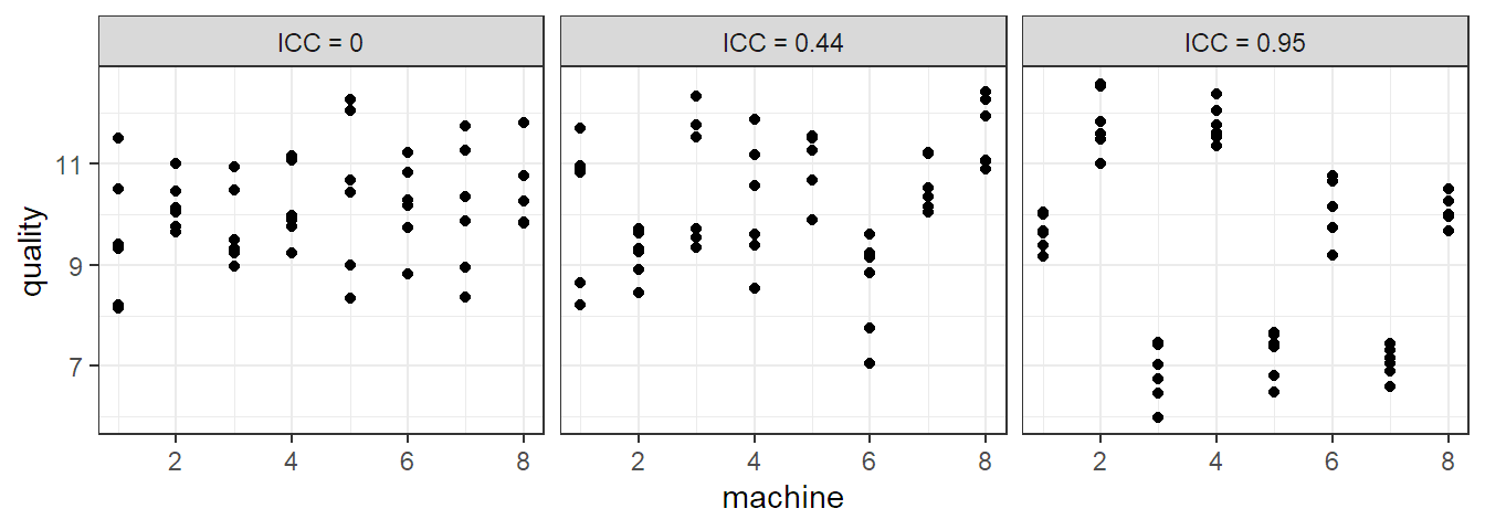
FIGURE 6.1: ICC value of three data sets of eight machines with six observations each.
This nonzero correlation within the same machine is in contrast to the fixed effects model (2.4), where all values are independent, because there, the \(\alpha_i\)’s are parameters, that is fixed, unknown quantities, and therefore also uncorrelated.
Parameter estimation for the variance components \(\sigma_{\alpha}^2\) and \(\sigma^2\) is nowadays typically being done with a technique called restricted maximum likelihood (REML), see for example Jiang and Nguyen (2021) for more details. We could also use classical maximum likelihood estimators here, but REML estimates are less biased. The parameter \(\mu\) is estimated with maximum likelihood assuming that the variances are known. Historically, method of moments estimators were (or are) also heavily used, see for example Kuehl (2000) or Oehlert (2000).
In R, there are many packages that can fit such models. We will consider
lme4 (Bates et al. 2015) and later also lmerTest (Kuznetsova, Brockhoff, and Christensen 2017), which
basically uses lme4 for model fitting and adds some statistical tests on
top.
Let us now consider Exercise 5.1 from Kuehl (2000) about an inheritance study with beef animals. Five sires, male animals, were each mated to a separate group of dams, female animals. The birth weights of eight male calves (from different dams) in each of the five sire groups were recorded. We want to find out what part of the total variation is due to variation between different sires. In fact, such random effects models were used very early in animal breeding programs, see for example Henderson (1963).
We first create the data set and visualize it.
## Create data set ####
weight <- c(61, 100,  56, 113,  99, 103,  75,  62,  ## sire 1
            75, 102,  95, 103,  98, 115,  98,  94,  ## sire 2
            58,  60,  60,  57,  57,  59,  54, 100,  ## sire 3
            57,  56,  67,  59,  58, 121, 101, 101,  ## sire 4
            59,  46, 120, 115, 115,  93, 105,  75)  ## sire 5
sire    <- factor(rep(1:5, each = 8))
animals <- data.frame(weight, sire)
str(animals)
## 'data.frame': 40 obs. of 2 variables:
## $ weight: num 61 100 56 113 99 103 ...
## $ sire : Factor w/ 5 levels "1","2","3","4",..: 1 1 1 1 1 1 ...
## Visualize data ####
stripchart(weight ~ sire, vertical = TRUE, pch = 1, xlab = "sire",
           data = animals)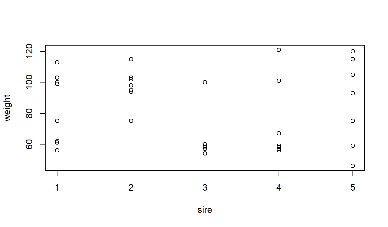
At first sight it looks like the variation between different sires is rather small.
Now we fit the random effects model with the lmer function in package lme4.
We want to have a random effect per sire. This can be specified with the
notation (1 | sire) in the model formula. This means that the “granularity” of
the random effect is specified after the vertical bar “|”. All observations
sharing the same level of sire will get the same random effect \(\alpha_i\). The
“1” means that we only want to have a so-called random intercept (\(\alpha_i\))
per sire. In the regression setup, we could also have a random slope for which
we would use the notation (x | sire) for a continuous predictor x. However,
this is not of relevance here.
As usual, the function summary gives an overview of the fitted model.
summary(fit.animals)## Linear mixed model fit by REML ['lmerMod']
## ...
## Random effects:
## Groups Name Variance Std.Dev.
## sire (Intercept) 117 10.8
## Residual 464 21.5
## Number of obs: 40, groups: sire, 5
##
## Fixed effects:
## Estimate Std. Error t value
## (Intercept) 82.55 5.91 14From the summary we can read off the table labelled Random Effects that \(\widehat{\sigma}_{\alpha}^2 = 117\) (sire) and
\(\widehat{\sigma}^2 = 464\) (Residual). Note that the column Std.Dev is
nothing more than the square root of the variance and not the standard
error (accuracy) of the variance estimate.
The variance of \(Y_{ij}\) is
therefore estimated as \(117 + 464 = 581\). Hence, only about \(117 / 581 = 20\%\) of the total
variance of the birth weight is due to sire, this is the intraclass
correlation. This confirms our visual inspection from above. It is good practice
to verify whether the grouping structure was interpreted
correctly. In the row Number of obs we can read off that we have 40
observations in total and a grouping factor given by sire which has five levels.
Under Fixed effects we find the estimate \(\widehat{\mu} = 82.55\).
It is an estimate for the expected birth weight of a male calf
of a randomly selected sire, randomly selected from the whole
population of all sires.
Approximate 95% confidence intervals for the parameters can be obtained with the function
confint (the argument oldNames has to bet set to FALSE to get a nicely
labelled output).
confint(fit.animals, oldNames = FALSE)## 2.5 % 97.5 %
## sd_(Intercept)|sire 0.00 24.62
## sigma 17.33 27.77
## (Intercept) 69.84 95.26Hence, an approximate 95% confidence interval for the standard deviation
\(\sigma_{\alpha}\) is given by \([0, \, 24.62]\). We see
that the estimate \(\widehat{\sigma}_{\alpha}\) is therefore quite
imprecise. The reason is that we only have five sires to estimate the
standard deviation. The corresponding confidence interval for the variance \(\sigma_{\alpha}^2\) would
be given by \([0^2, \, 24.62^2]\) (we can simply apply the square
function to the interval boundaries). The row labelled with (Intercept) contains the corresponding
confidence interval for \(\mu\).
What would happen if we used the “ordinary” aov function here?
options(contrasts = c("contr.sum", "contr.poly"))
fit.animals.aov <- aov(weight ~ sire, data = animals)
confint(fit.animals.aov)
## 2.5 % 97.5 %
## (Intercept) 75.637 89.463
## sire1 -12.751 14.901
## sire2 1.124 28.776
## sire3 -33.251 -5.599
## sire4 -18.876 8.776As we have used contr.sum, the confidence interval for \(\mu\) which can
be found under (Intercept) is a confidence interval for the average of
the expected birth weight of the male offsprings of these five specific
sires. More precisely, each of the five sires has its expected
birth weight \(\mu_i, i = 1, \ldots, 5\) (of a male offspring). With
contr.sum we have
\[
\mu = \frac{1}{5} \sum_{i=1}^g \mu_i,
\]
i.e., \(\mu\) is the average of the expected value of these five
specific sires. We see that this confidence interval is shorter than
the one from the random effects model. The reason is the different
interpretation. The random effects model allows to make inference about
the population of all sires (where we have seen five so far), while the
fixed effects model allows to make inference about these five specific
sires. Hence, we are facing a more difficult problem with the random
effects model; this is why we are less confident in our estimate
resulting in wider confidence intervals compared to the fixed effects
model.
We can also get “estimates” of the random effects \(\alpha_i\) with the function ranef.
ranef(fit.animals)## $sire
## (Intercept)
## 1 0.7183
## 2 9.9895
## 3 -12.9797
## 4 -3.3744
## 5 5.6462
##
## with conditional variances for "sire"More precisely, as the random effects are random quantities and not fixed
parameters, what we get with ranef are the conditional
means (given the observed data) which are the best
linear unbiased predictions, also
known as BLUPs (Robinson 1991). Typically, these estimates are shrunken
toward zero because of the normal assumption, hence we get slightly
different results compared to the fixed effects model. This is also known as the
so-called shrinkage property.
We should of course also check the model assumptions. Here, this includes in
addition normality of the random effects, though this is hard to check with only
five observations. We get the Tukey-Anscombe plot
with the plot function.
plot(fit.animals) ## TA-plot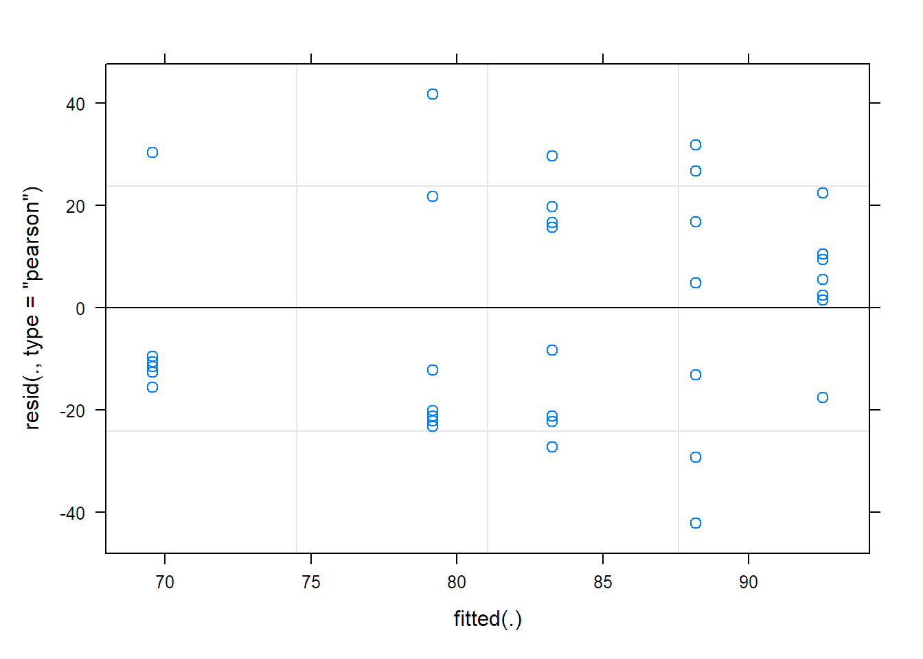
To get QQ-plots of the random effects and the residuals, we need to
extract them first and then use qqnorm as usual.
par(mfrow = c(1, 2))
qqnorm(ranef(fit.animals)$sire[,"(Intercept)"],
       main = "Random effects")
qqnorm(resid(fit.animals), main = "Residuals")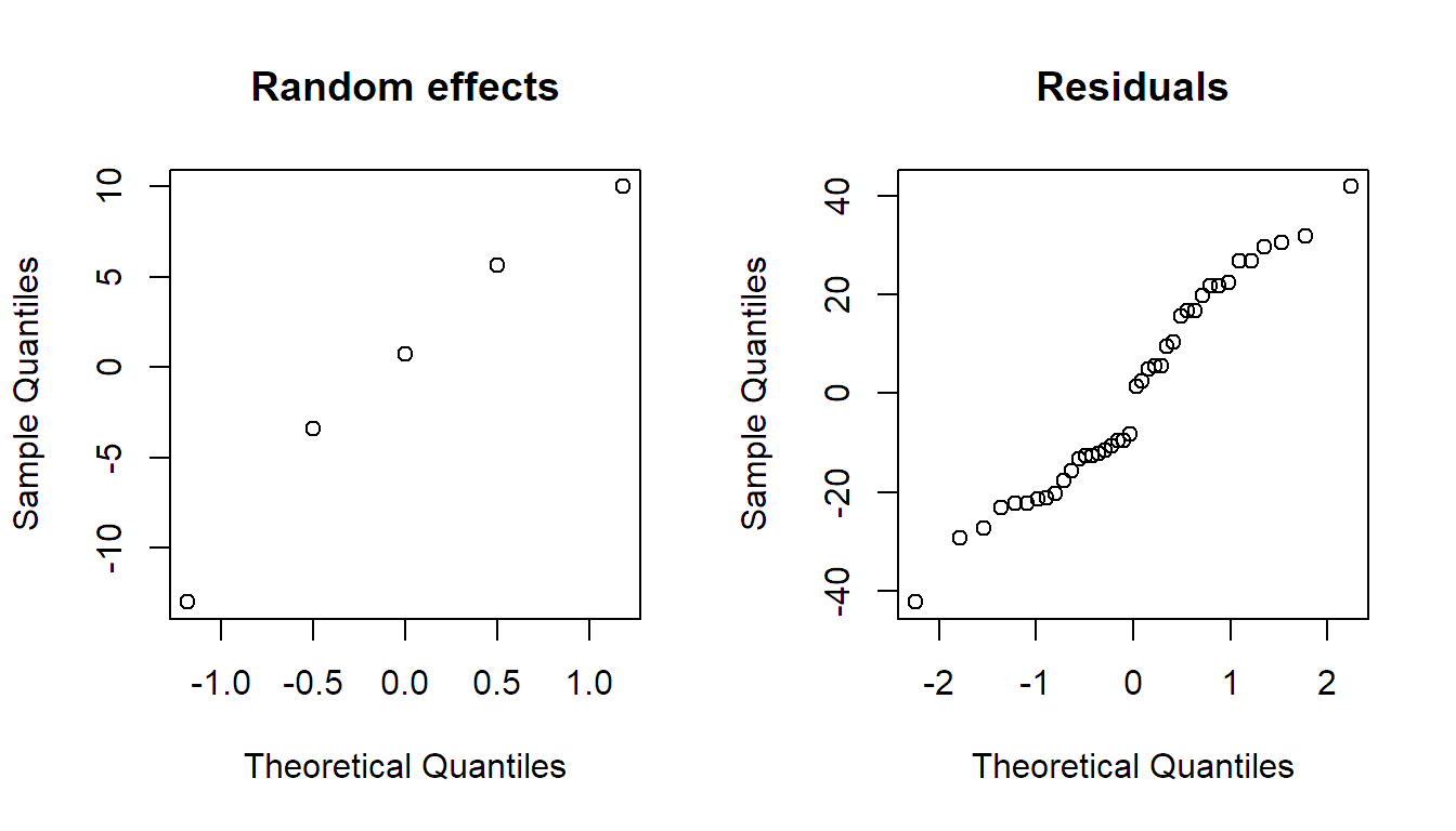
Depending on the model complexity, residual analysis for models including random
effects can be subtle, this includes the models we will learn about in Section
6.2 too, see for example Santos Nobre and Motta Singer (2007),
Loy and Hofmann (2015) or Loy, Hofmann, and Cook (2017). Some implementations of these papers can be found in
package HLMdiag (Loy and Hofmann 2014).
Sometimes you also see statistical tests of the form \(H_0: \sigma_{\alpha} = 0\)
vs. \(H_A: \sigma_{\alpha} > 0\). For model (6.1) we could
actually get exact p-values, while for complex models later this is not the case
anymore. In these situations, approximate or simulation based methods have to be used. Some
can be found in package RLRsim (Scheipl, Greven, and Kuechenhoff 2008).
6.1.2 More Than One Factor
So far this was a one-way ANOVA model with a random effect. We can extend this to the two-way ANOVA situation and beyond. For this reason, we consider the following example:
A large company randomly selected five employees and six batches of source material from the production process. The material from each batch was divided into 15 pieces which were randomized to the different employees such that each employee would build three test specimens from each batch. The response was the corresponding quality score. The goal was to quantify the different sources of variation.
We first load the data and get an overview.
book.url <- "https://stat.ethz.ch/~meier/teaching/book-anova"
quality <- readRDS(url(file.path(book.url, "data/quality.rds")))
str(quality)
## 'data.frame': 90 obs. of 3 variables:
## $ employee: Factor w/ 5 levels "1","2","3","4",..: 1 1 1 1 1 1 ...
## $ batch : Factor w/ 6 levels "B1","B2","B3",..: 1 1 1 2 2 2 ...
## $ score : num 27.4 27.8 27.3 25.5 25.5 26.4 ...
xtabs(~ batch + employee, data = quality)## employee
## batch 1 2 3 4 5
## B1 3 3 3 3 3
## B2 3 3 3 3 3
## B3 3 3 3 3 3
## B4 3 3 3 3 3
## B5 3 3 3 3 3
## B6 3 3 3 3 3We can for example visualize this data set with an interaction plot.
with(quality, interaction.plot(x.factor = batch,
                               trace.factor = employee,
                               response = score))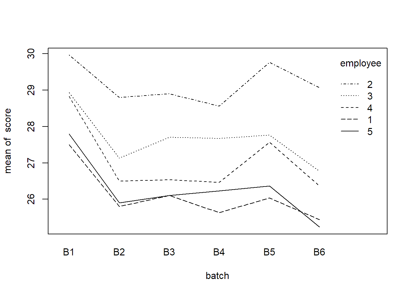
There seems to be variation between different employees and between the different batches. The interaction does not seem to be very pronounced. Let us set up a model for this data. We denote the observed quality score of the \(k\)th sample of employee \(i\) using material from batch \(j\) by \(y_{ijk}\). A natural model is then \[\begin{equation} Y_{ijk} = \mu + \alpha_i + \beta_j + (\alpha\beta)_{ij} + \epsilon_{ijk}, \tag{6.2} \end{equation}\] where \(\alpha_i\) is the random (main) effect of employee \(i\), \(\beta_j\) is the random (main) effect of batch \(j\), \((\alpha\beta)_{ij}\) is the random interaction term between employee \(i\) and batch \(j\) and \(\epsilon_{ijk} \textrm{ i.i.d.} \sim N(0, \sigma^2)\) is the error term. For the random effects we have the usual assumptions \[\begin{align*} \alpha_i & \textrm{ i.i.d.} \sim N(0, \sigma_{\alpha}^2), \\ \beta_j & \textrm{ i.i.d.} \sim N(0, \sigma_{\beta}^2), \\ (\alpha\beta)_{ij} & \textrm{ i.i.d.} \sim N(0, \sigma_{\alpha\beta}^2). \end{align*}\] In addition, we assume that \(\alpha_i\), \(\beta_j\), \((\alpha\beta)_{ij}\) and \(\epsilon_{ijk}\) are independent. As each random term in the model has its own variance component, we now have the variances \(\sigma_{\alpha}^2\), \(\sigma_{\beta}^2\), \(\sigma_{\alpha\beta}^2\) and \(\sigma^2\).
What is the interpretation of the different terms? The random (main) effect of employee is the variability between different employees, and the random (main) effect of batch is the variability between different batches. The random interaction term can for example be interpreted as quality inconsistencies of employees across different batches.
Let us fit such a model in R. We want to have a random effect per employee (=
(1 | employee)), a random effect per batch (= (1 | batch)), and a random
effect per combination of employee and batch (= (1 | employee:batch)).
fit.quality <- lmer(score ~ (1 | employee) + (1 | batch) +
                      (1 | employee:batch), data = quality)
summary(fit.quality)
## Linear mixed model fit by REML ['lmerMod']
## ...
## Random effects:
## Groups Name Variance Std.Dev.
## employee:batch (Intercept) 0.0235 0.153
## batch (Intercept) 0.5176 0.719
## employee (Intercept) 1.5447 1.243
## Residual 0.2266 0.476
## Number of obs: 90, groups: employee:batch, 30; batch, 6; employee, 5
##
## Fixed effects:
## Estimate Std. Error t value
## (Intercept) 27.248 0.631 43.2From the output we get \(\widehat{\sigma}_{\alpha}^2 = 1.54\) (employee), \(\widehat{\sigma}_{\beta}^2 = 0.52\) (batch), \(\widehat{\sigma}_{\alpha\beta}^2 = 0.02\) (interaction of employee and batch) and \(\widehat{\sigma}^2 = 0.23\) (error term).
Hence, total variance is \(1.54 + 0.52 + 0.02 + 0.23 = 2.31\). We see that the largest contribution to the variance
is variability between different employees which contributes to about
\(1.54 / 2.31 \approx 67\%\)
of the total variance. These are all point estimates. Confidence intervals on
the scale of the standard deviations can be obtained by calling confint.
confint(fit.quality, oldNames = FALSE)## 2.5 % 97.5 %
## sd_(Intercept)|employee:batch 0.0000 0.3528
## sd_(Intercept)|batch 0.4100 1.4754
## sd_(Intercept)|employee 0.6694 2.4994
## sigma 0.4020 0.5741
## (Intercept) 25.9190 28.5766Uncertainty is quite large. In addition, there is no statistical evidence that the random interaction term is really needed, as the corresponding confidence interval contains zero. To get a more narrow confidence interval for the standard deviation between different employees, we would need to sample more employees. Basically, each employee contributes one observation for estimating the standard deviation (or variance) between employees. The same reasoning applies to batch.
6.1.3 Nesting
To introduce a new concept, we consider the Pastes data set in package lme4.
The strength of a chemical paste product was measured for a total of 30
samples coming from 10 randomly selected delivery batches where each
contained three randomly selected casks. Each sample was measured twice, resulting
in a total of 60 observations. We want to check what part of the total
variability of strength is due to variability between batches, between casks and
due to measurement error.
## 'data.frame':    60 obs. of  4 variables:
##  $ strength: num  62.8 62.6 60.1 62.3 62.7 63.1 ...
##  $ batch   : Factor w/ 10 levels "A","B","C","D",..: 1 1 1 1 1 1 ...
##  $ cask    : Factor w/ 3 levels "a","b","c": 1 1 2 2 3 3 ...
##  $ sample  : Factor w/ 30 levels "A:a","A:b","A:c",..: 1 1 2 2 3 3 ...
Note that the levels of batch and cask are given by upper- and lowercase
letters, respectively. If we carefully think about the data structure, we have
just discovered a new way of combining factors. Cask a in batch A has
nothing to do with cask a in batch B and so on. The level a of cask has
a different meaning for every level of batch. Hence, the two factors cask
and batch are not crossed. We say cask is
nested in batch. The data set also
contains an additional (redundant) factor sample which is a unique identifier
for each sample, given by the combination of batch and cask.
We use package ggplot2 to visualize the data set (R code for interested
readers only). The different panels are the different batches (A to J).
library(ggplot2)
ggplot(Pastes, aes(y = cask, x = strength)) + geom_point() +
  facet_grid(batch ~ .)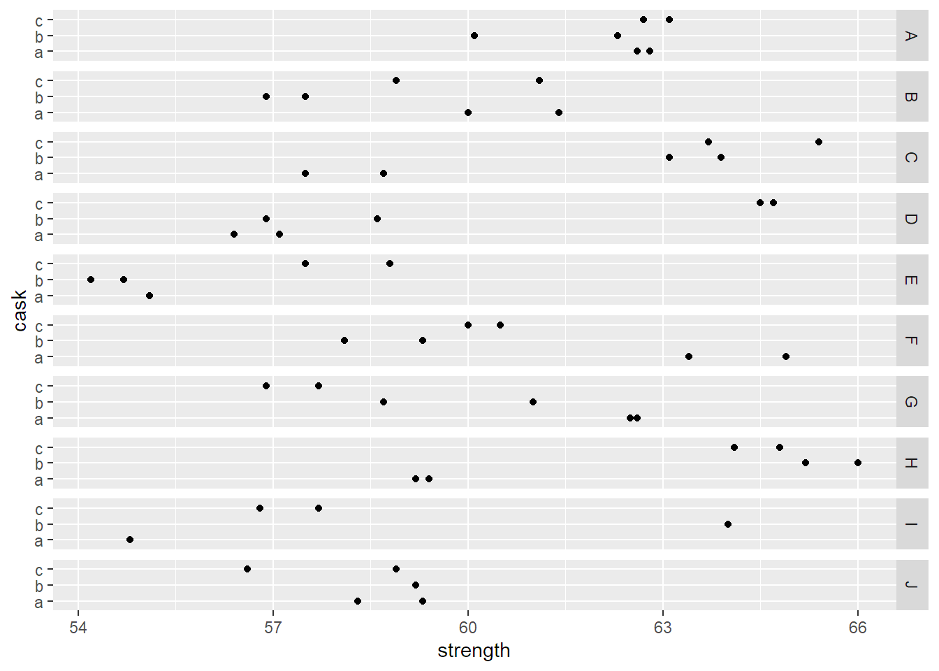
The batch effect does not seem to be very pronounced, for example, there is no clear tendency that some batches only contain large values, while others only contain small values. Casks within the same batch can be substantially different, but the two measurements from the same cask are typically very similar. Let us now set up an appropriate random effects model for this data set.
Let \(y_{ijk}\) be the observed strength of the \(k\)th sample of cask \(j\) in batch \(i\). We can then use the model \[\begin{equation} Y_{ijk} = \mu + \alpha_i + \beta_{j(i)} + \epsilon_{ijk}, \tag{6.3} \end{equation}\] where \(\alpha_i\) is the random effect of batch and \(\beta_{j(i)}\) is the random effect of cask within batch. Note the special notation \(\beta_{j(i)}\) which emphasizes that cask is nested in batch. This means that each batch gets its own coefficient for the cask effect (from a technical point of view this is like an interaction effect without the corresponding main effect). We make the usual assumptions for the random effects \[ \alpha_i \, \textrm{ i.i.d.} \sim N(0, \sigma_{\alpha}^2), \quad \beta_{j(i)} \, \textrm{ i.i.d.} \sim N(0, \sigma_{\beta}^2), \] and similarly for the error term \(\epsilon_{ijk} \sim N(0, \sigma^2)\). As before, we assume independence between all random terms.
We have to tell lmer about the nesting structure. There are multiple ways to
do so. We can use the notation (1 | batch/cask) which means that we want to
have a random effect per batch and per cask within batch. We could also use
(1 | batch) + (1 | cask:batch) which means that we want to have a random
effect per batch and a random effect per combination of batch and cask, which
is the same as a nested effect. Last but not least, here we could also use (1 | batch) + (1 | sample). Why? Because sample is the combination of batch
and cask. Note that we cannot use the notation (1 | batch) + (1 | cask)
here because then for example all casks a (across different batches) would
share the same effect (similar for the other levels of cask). This is not what
we want.
Let us fit a model using the notation (1 | batch/cask).
## Linear mixed model fit by REML ['lmerMod']
## ...
## Random effects:
##  Groups     Name        Variance Std.Dev.
##  cask:batch (Intercept) 8.434    2.904
##  batch      (Intercept) 1.657    1.287
##  Residual               0.678    0.823
## Number of obs: 60, groups:  cask:batch, 30; batch, 10
##
## Fixed effects:
##             Estimate Std. Error t value
## (Intercept)   60.053      0.677    88.7
We have \(\widehat{\sigma}_{\alpha}^2 = 1.66\) (batch),
\(\widehat{\sigma}_{\beta}^2 = 8.43\) (cask) and \(\widehat{\sigma}^2 = 0.68\) (measurement error). This confirms that most variation is in
fact due to cask within batch. Confidence intervals could be obtained as usual
with the function confint (not shown).
A nested effect has also some associated degrees of freedom. In the previous example, cask has 3 levels in each of the 10 batches. The reasoning is now as follows: As cask needs 2 degrees of freedom in each level of the 10 batches, the degrees of freedom of cask are \(10 \cdot 2 = 20\).
6.2 Mixed Effects Models
In practice, we often encounter models which contain both random and fixed effects. We call them mixed models or mixed effects models.
6.2.1 Example: Machines Data
We start with the data set Machines in package nlme (Pinheiro et al. 2021). As stated
in the help file: “Data on an experiment to compare three brands of machines
used in an industrial process […]. Six workers were chosen randomly among the
employees of a factory to operate each machine three times. The response is an
overall productivity score taking into account the number and quality of
components produced.”
data("Machines", package = "nlme")
## technical details for shorter output:
class(Machines) <- "data.frame"
Machines[, "Worker"] <- factor(Machines[, "Worker"], levels = 1:6,
                               ordered = FALSE)
str(Machines, give.attr = FALSE) ## give.attr to shorten output
## 'data.frame': 54 obs. of 3 variables:
## $ Worker : Factor w/ 6 levels "1","2","3","4",..: 1 1 1 2 2 2 ...
## $ Machine: Factor w/ 3 levels "A","B","C": 1 1 1 1 1 1 ...
## $ score : num 52 52.8 53.1 51.8 52.8 53.1 ...Let us first visualize the data. In addition to plotting all individual data, we
also calculate the mean for each combination of worker and machine and connect
these values with lines for each worker (R code for interested readers only).
ggplot(Machines, aes(x = Machine, y = score, group = Worker, col = Worker)) +
  geom_point() + stat_summary(fun = mean, geom = "line") + theme_bw()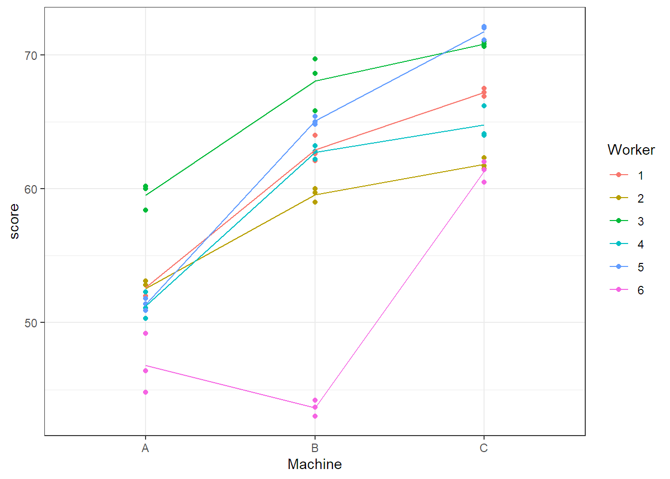
## A classical interaction plot would be (not shown)
with(Machines, interaction.plot(x.factor = Machine,
                                trace.factor = Worker,
                                response = score))
We observe that on average, productivity is largest on machine C, followed by B
and A. Most workers show a similar profile, with the exception of
worker 6 who performs badly on machine B.
Let us now try to model this data. The goal is to make inference about the specific machines at hand, this is why we treat machine as a fixed effect. We assume that there is a population machine effect (think of an average profile across all potential workers), but each worker is allowed to have its own random deviation. With \(y_{ijk}\) we denote the observed \(k\)th productivity score of worker \(j\) on machine \(i\). We use the model \[\begin{equation} Y_{ijk} = \mu + \alpha_i + \beta_j + (\alpha\beta)_{ij} + \epsilon_{ijk}, \tag{6.4} \end{equation}\] where \(\alpha_i\) is the fixed effect of machine \(i\) (with a usual side constraint), \(\beta_j\) is the random effect of worker \(j\) and \((\alpha\beta)_{ij}\) is the corresponding random interaction effect. An interaction effect between a random (here, worker) and a fixed effect (here, machine) is treated as a random effect.
What is the interpretation of this model? The average (over the whole population) productivity profile with respect to the three different machines is given by the fixed effect \(\alpha_i\). The random deviation of an individual worker consists of a general shift \(\beta_j\) (worker specific general productivity level) and a worker specific preference \((\alpha\beta)_{ij}\) with respect to the three machines. We assume that all random effects are normally distributed, this means \[ \beta_j \, \textrm{ i.i.d.} \sim N(0, \sigma_{\beta}^2), \quad (\alpha\beta)_{ij} \, \textrm{ i.i.d.} \sim N(0, \sigma_{\alpha\beta}^2). \] For the error term we assume as always \(\epsilon_{ijk} \, \textrm{ i.i.d.} \sim N(0, \sigma^2)\). In addition, all random terms are assumed to be independent.
We visualize model (6.4) step-by-step in Figure 6.2. The solid line is the population average of the machine effect \((= \mu + \alpha_i)\), the dashed line is the population average including the worker specific general productivity level \((= \mu + \alpha_i + \beta_j)\), i.e., a parallel shift of the solid line. The dotted line in addition includes the worker specific machine preference \((= \mu + \alpha_i + \beta_j + (\alpha\beta)_{ij})\). Individual observations of worker \(j\) now fluctuate around these values.
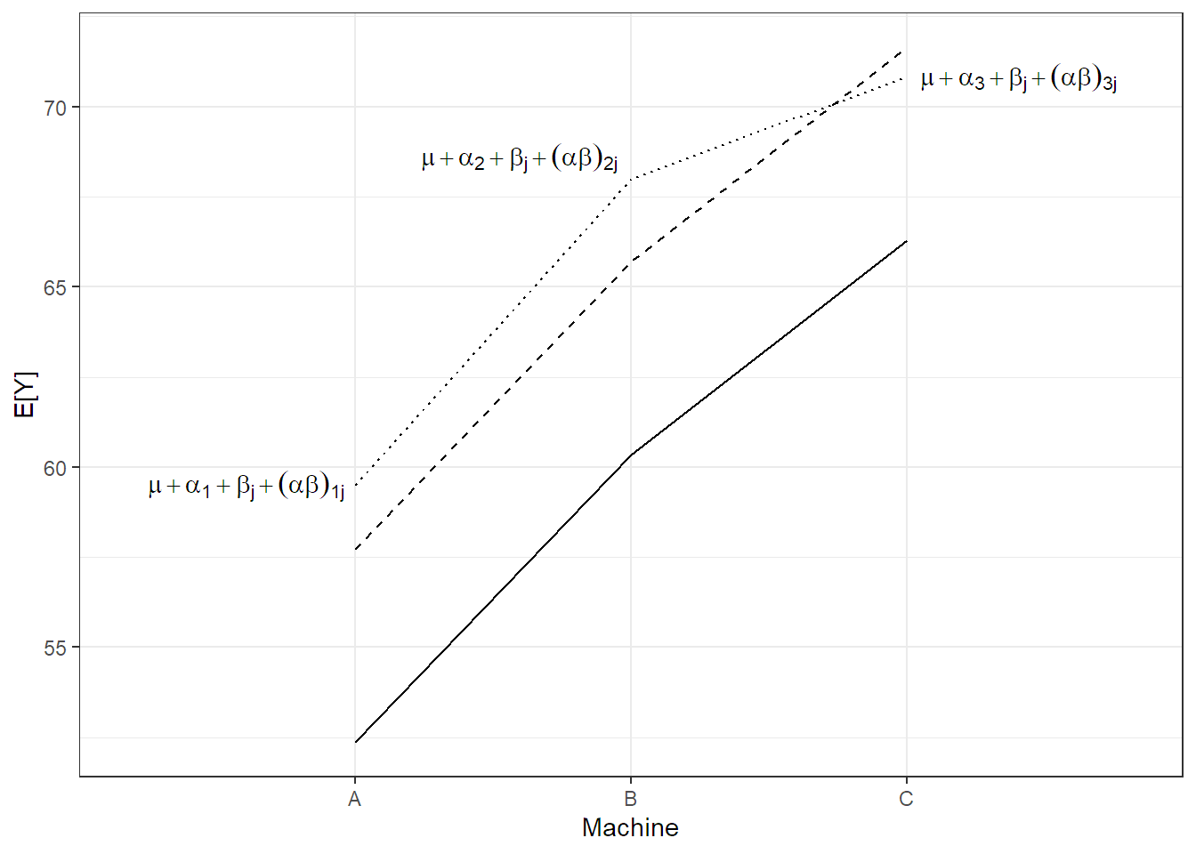
FIGURE 6.2: Illustration of model (6.4) for the machines data set.
We could use the lme4 package to fit such a model. Besides the fixed effect of
machine type we want to have the following random effects:
- a random effect \(\beta_j\) per worker:
(1 | Worker) - a random effect \((\alpha\beta)_{ij}\) per combination of worker and machine:
(1 | Worker:Machine)
Hence, the lmer call would look as follows.
fit.machines <- lmer(score ~ Machine + (1 | Worker) +
                       (1 | Worker:Machine), data = Machines)
As lme4 does not calculate p-values for the fixed effects, we use the
package lmerTest instead. Technically speaking, lmerTest uses lme4 to fit
the model and then adds some statistical tests, i.e., p-values for the fixed
effects, to the output. There are still many open issues regarding statistical
inference in mixed models, see for example the “GLMM
FAQ” (the so-called
generalized linear mixed models frequently asked questions). However, for “nice”
designs (as the current one), we get proper statistical inference using the
lmerTest package.
options(contrasts = c("contr.treatment", "contr.poly"))
library(lmerTest)
fit.machines <- lmer(score ~ Machine + (1 | Worker) +
                       (1 | Worker:Machine), data = Machines)
We get the ANOVA table for the fixed effects with the function anova.
anova(fit.machines)## Type III Analysis of Variance Table with Satterthwaite's method
## Sum Sq Mean Sq NumDF DenDF F value Pr(>F)
## Machine 38.1 19 2 10 20.6 0.00029The fixed effect of machine is significant. If we closely inspect the output,
we see that an \(F\)-distribution with 2 and 10 degrees of freedom is being used.
Where does the value 10 come from? It seems to be a rather small number given
the sample size of 54 observations. Let us remind ourselves what the fixed
effect actually means. It is the average machine effect, where the average is
taken over the whole population of workers (where we have seen only six). We
know that every worker has its own random deviation of this effect. Hence, the
relevant question is whether the worker profiles just fluctuate around a
constant machine effect (all \(\alpha_i = 0\)) or whether the machine effect is
substantially larger than this worker specific machine variation. Technically
speaking, the worker specific machine variation is nothing more than the
interaction between worker and machine. Hence, this boils down to comparing
the variation between different machines (having 2 degrees of freedom) to the
variation due to the interaction between machines and workers (having \(2 \cdot 5 = 10\) degrees of freedom). The lmerTest package automatically detects this
because of the structure of the random effects. This way of thinking also allows
another insight: If we want the estimate of the population average of the
machine effect (the fixed effect of machine) to have a desired accuracy, the
relevant quantity to increase is the number of workers.
If we call summary on the fitted object, we get the individual
\(\widehat{\alpha}_i\)’s under Fixed effects.
summary(fit.machines)## Linear mixed model fit by REML. t-tests use Satterthwaite's method [
## lmerModLmerTest]
## ...
## Random effects:
## Groups Name Variance Std.Dev.
## Worker:Machine (Intercept) 13.909 3.730
## Worker (Intercept) 22.858 4.781
## Residual 0.925 0.962
## Number of obs: 54, groups: Worker:Machine, 18; Worker, 6
##
## Fixed effects:
## Estimate Std. Error df t value Pr(>|t|)
## (Intercept) 52.36 2.49 8.52 21.06 1.2e-08
## MachineB 7.97 2.18 10.00 3.66 0.0044
## MachineC 13.92 2.18 10.00 6.39 7.9e-05
## ...Let us first check whether the structure was interpreted correctly
(Number of obs): There are 54 observations, coming from 6 different workers
and 18 (\(=3 \cdot 6\)) different combinations of workers and machines.
As usual, we have to be careful with the interpretation of the fixed effects
because it depends on the side constraint that is being used. For example, here
we can read off the output that the productivity score on machine B is on
average 7.97 units larger than on machine A . We can
also get the parameter estimates of the fixed effects only by calling
fixef(fit.machines) (not shown).
Estimates of the different variance components can be found under
Random effects. Often, we are not very much interested in the actual
values. We rather use the random effects as a “tool” to model correlated data
and to tell the fitting function that we are interested in the
population average and not the worker specific machine effects. In that
sense, including random effects in a model changes the interpretation of
the fixed effects. Hence, it really depends on the research question
whether we treat a factor as fixed or random. There is no right or wrong
here.
Approximate 95% confidence intervals can be obtained as usual with the
function confint.
confint(fit.machines, oldNames = FALSE)## 2.5 % 97.5 %
## sd_(Intercept)|Worker:Machine 2.353 5.432
## sd_(Intercept)|Worker 1.951 9.411
## sigma 0.776 1.235
## (Intercept) 47.395 57.316
## MachineB 3.738 12.195
## MachineC 9.688 18.145For example, a 95% confidence interval for the expected value of the
difference between machine A and B is given by
\([3.7, 12.2]\).
We can do the residual analysis as outlined in Section 6.1.1.
## Tukey-Anscombe plot
plot(fit.machines)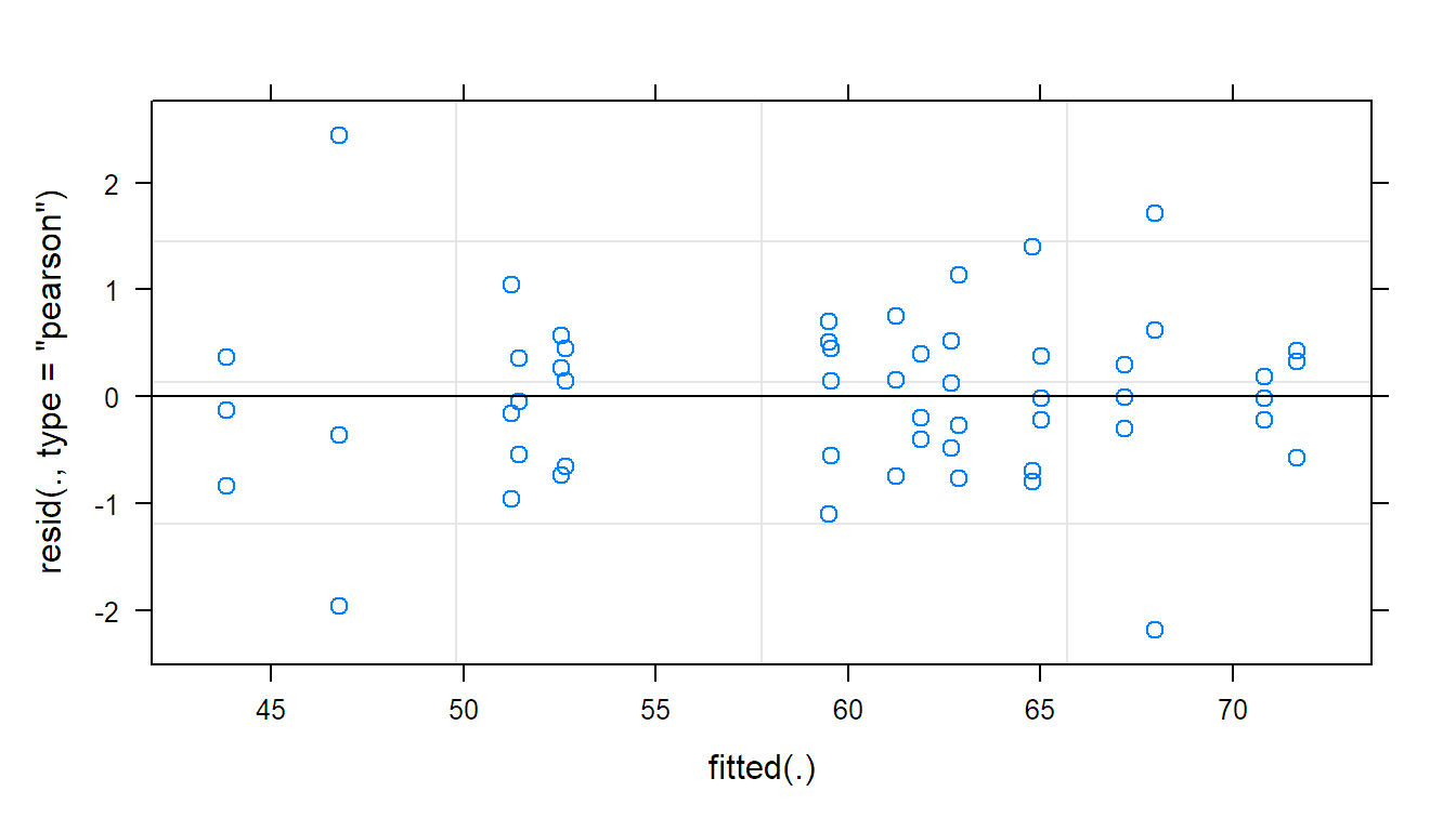
## QQ-plots
par(mfrow = c(1, 3))
qqnorm(ranef(fit.machines)$Worker[, 1],
       main = "Random effects of worker")
qqnorm(ranef(fit.machines)$'Worker:Machine'[, 1],
       main = "Random interaction")
qqnorm(resid(fit.machines), main = "Residuals")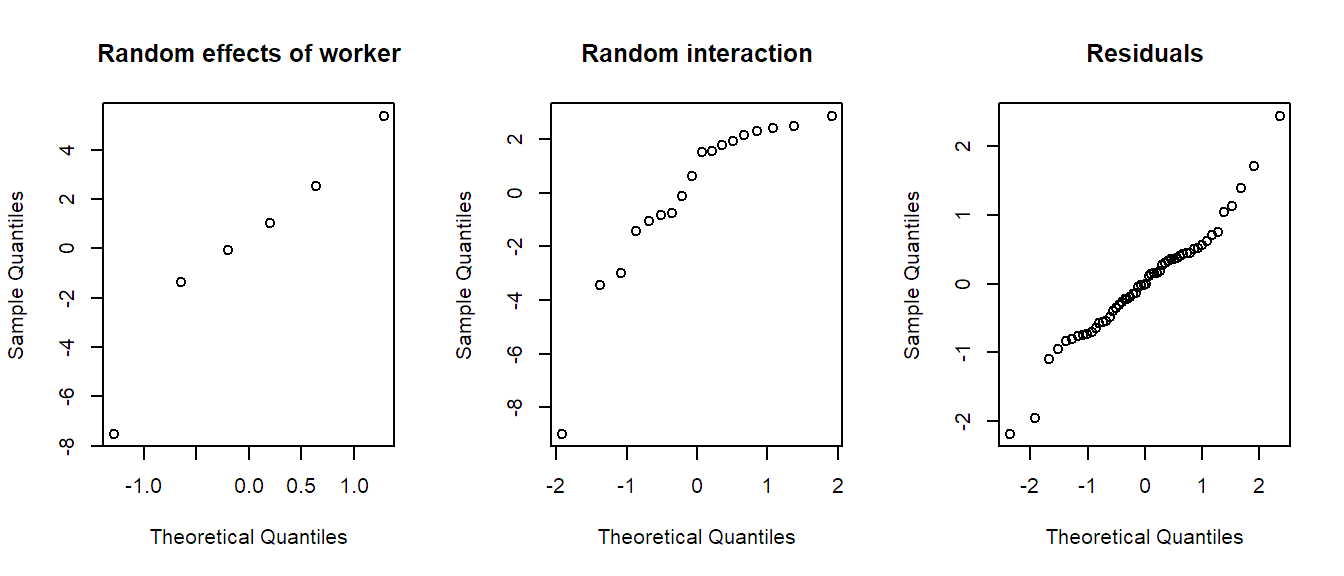
The Tukey-Anscombe plot looks good. The QQ-plots could look better; however, we do not have a lot of observations such that the deviations are still OK. Or in other words, it is difficult to detect clear violations of the normality assumption.
Again, in order to better understand the mixed model, we check what happens if we would fit a purely fixed effects model here. We use sum-to-zero side constraints in the following interpretation.
##                Df Sum Sq Mean Sq F value Pr(>F)
## Machine         2   1755     878   949.2 <2e-16
## Worker          5   1242     248   268.6 <2e-16
## Machine:Worker 10    427      43    46.1 <2e-16
## Residuals      36     33       1
The machine effect is much more significant. This is because in the fixed effects model, the main effect of machine makes a statement about the average machine effect of these 6 specific workers and not about the population average (in the same spirit as in the sire example in Section 6.1.1).
Remark: The model in Equation (6.4) with
\((\alpha\beta)_{ij} \, \textrm{ i.i.d.} \sim N(0, \sigma_{\alpha\beta}^2)\) is
also known as the so-called unrestricted model.
There is also a restricted model where we would
assume that a random interaction effect sums up to zero if we sum over the
fixed indices. For our example this would mean that if we sum up the interaction
effect for each worker across the different machines, we would get zero. Here,
the restricted model means that the random interaction term
does not contain any information about the general productivity level of a
worker, just about machine preference. Unfortunately, the restricted model is
currently not implemented in lmer. Luckily, the inference with respect to the
fixed effects is the same for both models, only the estimates of the variance
components differ. For more details, see for example Burdick and Graybill (1992).
6.2.2 Example: Chocolate Data
We continue with a more complex design which is a relabelled version of Example 12.2 of Oehlert (2000) (with some simulated data). A group of 10 raters with rural background and 10 raters with urban background rated 4 different chocolate types. Every rater tasted and rated two samples from the same chocolate type in random order. Hence, we have a total of \(20 \cdot 4 \cdot 2 = 160\) observations.
book.url <- "http://stat.ethz.ch/~meier/teaching/book-anova"
chocolate <- read.table(file.path(book.url, "data/chocolate.dat"),
                        header = TRUE)
chocolate[,"rater"]      <- factor(chocolate[,"rater"])
chocolate[,"background"] <- factor(chocolate[,"background"])
str(chocolate)
## 'data.frame': 160 obs. of 4 variables:
## $ choc : chr "A" "A" ...
## $ rater : Factor w/ 10 levels "1","2","3","4",..: 1 1 1 1 1 1 ...
## $ background: Factor w/ 2 levels "rural","urban": 1 1 1 1 1 1 ...
## $ y : int 61 64 46 45 63 66 ...Chocolate type is available in factor choc (with levels A, B, C and
D), background of rater (with levels rural and urban) in background, the
score in y and a rater ID can be found in rater. Note that the factor
rater has only 10 levels. We have to be careful here and should not forget
that rater is actually nested in background; so, the raters labelled 1 in
the urban and the rural group have nothing in common.
We can easily visualize this data with an interaction plot. We use the package
ggplot2 to get a more appealing plot compared to the
function interaction.plot (R code for interested readers only).
ggplot(chocolate, aes(x = choc, y = y,
                      group = interaction(background, rater),
                      color = background)) +
  stat_summary(fun = mean, geom = "line") + theme_bw()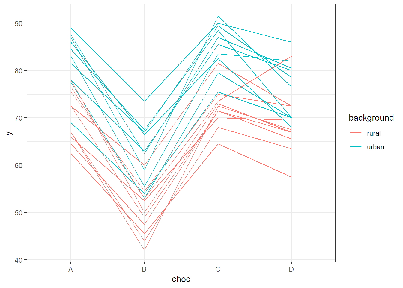
FIGURE 6.3: Interaction plot of the chocolate data set.
Questions that could arise are:
- Is there a background effect (urban vs. rural)?
- Is there a chocolate type effect?
- Does the effect of chocolate type depend on background (interaction)?
- How large is the variability between different raters regarding general chocolate liking level?
- How large is the variability between different raters regarding chocolate type preference?
Here, background and chocolate type are fixed effects, as we want to make a statement about these specific levels. However, we treat rater as random, as we want the fixed effects to be population average effects and we are interested in the variation between different raters.
We can use the model \[\begin{equation} Y_{ijkl} = \mu + \alpha_i + \beta_j + (\alpha\beta)_{ij} + \delta_{k(i)} + (\beta\delta)_{jk(i)} + \epsilon_{ijkl}, \tag{6.5} \end{equation}\] where
- \(\alpha_i\) is the (fixed) effect of background, \(i = 1, 2\),
- \(\beta_j\) is the (fixed) effect of chocolate type, \(j = 1, \ldots, 4\),
- \((\alpha\beta)_{ij}\) is the corresponding interaction (fixed effect),
- \(\delta_{k(i)}\) is the random effect of rater: “general chocolate liking level of rater \(k(i)\) (nested in background!)”, \(k = 1, \ldots, 10\),
- \((\beta\delta)_{jk(i)}\) is the (random) interaction of rater and chocolate type: “specific chocolate type preference of rater \(k(i)\)”.
We use the usual assumptions for all random terms. In this setup, for both backgrounds there is (over the whole population) an average preference profile with respect to the 4 different chocolate types (given by \(\mu + \alpha_i + \beta_j + (\alpha\beta)_{ij}\)). Every rater can have its individual random deviation from this profile. This deviation consists of a general shift \(\delta_{k(i)}\) (general chocolate liking of a rater) and a rater specific preference \((\beta\delta)_{jk(i)}\) with respect to the 4 chocolate types. This is visualized in Figure 6.4 (for urban raters only, \(i = 2\)). The situation is very similar to the previous example about machines in Section 6.2.1. The solid line is the population average \((= \mu + \alpha_2 + \beta_j + (\alpha\beta)_{2j})\). The dashed line is a parallel shift including the rater specific general chocolate liking level \((= \mu + \alpha_2 + \beta_j + (\alpha\beta)_{2j} + \delta_{k(2)})\). The dotted line in addition includes the rater specific chocolate type preference \((\mu + \alpha_2 + \beta_j + (\alpha\beta)_{2j} + \delta_{k(2)} + (\beta\delta)_{jk(2)})\). Therefore, the fixed effects have to be interpreted as population averages.
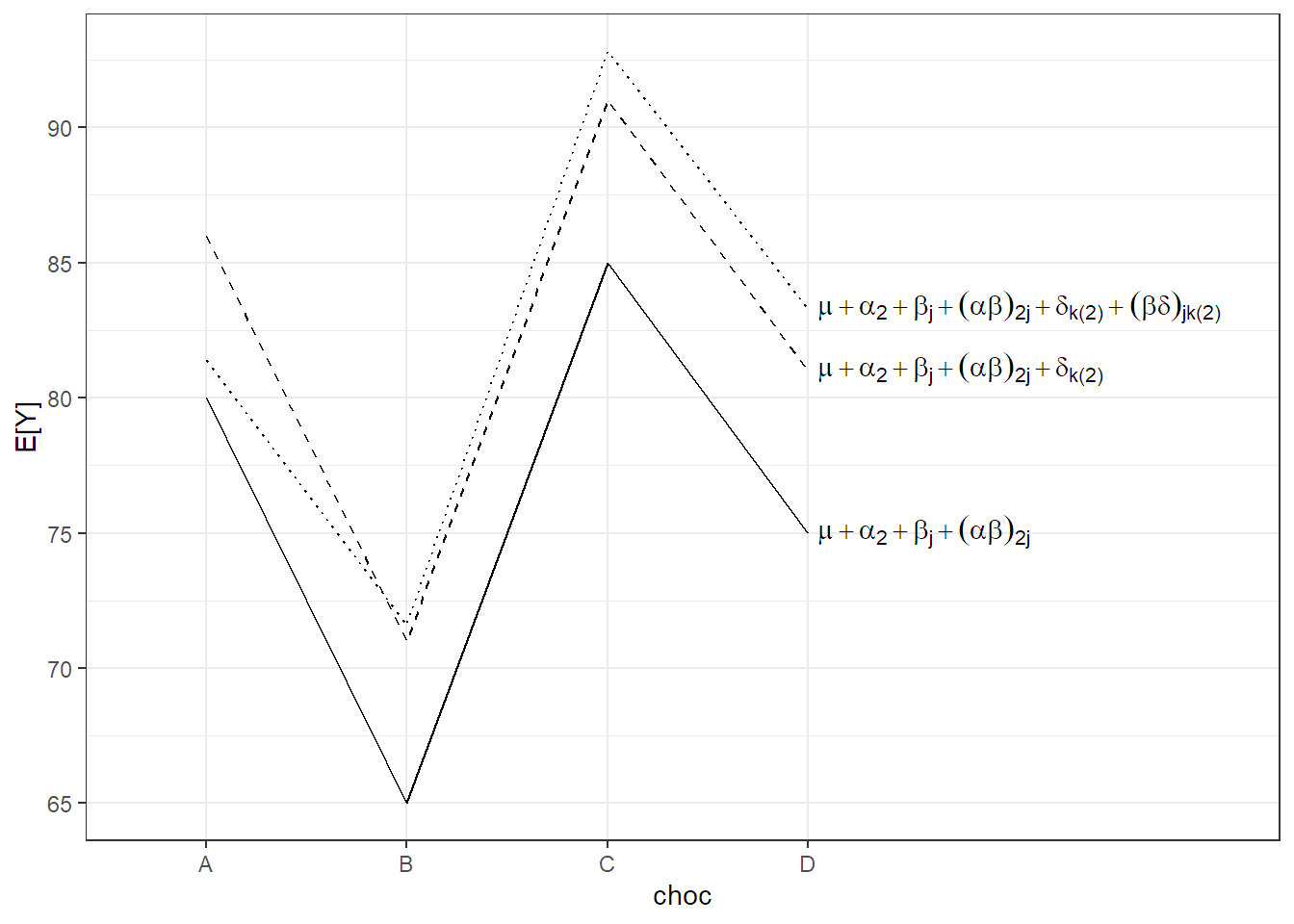
FIGURE 6.4: Illustration of model (6.5) for the chocolate data set for urban raters.
Let us now try to fit this model in R. We want to have
- main effects and the interaction for the fixed effects of background
and chocolate type:
background * choc - a random effect per rater (nested in background):
(1 | rater:background) - a random effect per chocolate type and rater (nested in background):
(1 | rater:background:choc).
We always write rater:background to get a unique rater ID. An
alternative would be to define another factor in the data set which
enumerates the raters from 1 to 20 (instead from 1 to 10).
Hence, the lmer call (using package lmerTest) looks as follows.
fit.choc <- lmer(y ~ background * choc + (1 | rater:background) +
                   (1 | rater:background:choc), data = chocolate)
As before, we get an ANOVA table with p-values for the fixed effects with the
function anova.
anova(fit.choc)## Type III Analysis of Variance Table with Satterthwaite's method
## Sum Sq Mean Sq NumDF DenDF F value Pr(>F)
## background 263 263 1 18 27.61 5.4e-05
## choc 4219 1406 3 54 147.74 < 2e-16
## background:choc 64 21 3 54 2.24 0.094We see that the interaction is not significant but both main effects are. This is what we already observed in the interaction plot in Figure 6.3. There, the profiles were quite parallel, but raters with an urban background rated higher on average than those with a rural background. In addition, there was a clear difference between different chocolate types.
Can we get an intuitive idea about the denominator degrees of freedom that are being used in these tests?
- The main effect of background can be thought of as a two-sample \(t\)-test with two groups having 10 observations each. Think of taking one average value per rater. Hence, we get \(2 \cdot 10 - 2 = 18\) degrees of freedom.
- As we allow for a rater specific chocolate type preference, we have to check whether the effect of chocolate is substantially larger than this rater specific variation. The rater specific variation can be thought of as the interaction between rater and chocolate type. As rater is nested in background, rater has 9 degrees of freedom in each background group. Hence, the interaction has (\((9 + 9) \cdot 3 = 54\)) degrees of freedom.
- The same argument as above holds true for the interaction between background and chocolate type.
Hence, if we want to get a more precise view about these population average effects, the relevant quantity to increase is the number of raters.
Approximate confidence intervals for the individual coefficients of the
fixed effects and the variance components could again be obtained by calling
confint(fit.choc, oldNames = FALSE) (output not shown).
Most often, the focus is not on the actual values of the variance components. We use these random effects to change the meaning of the fixed effects. By incorporating the random interaction effect between rater and chocolate type, the meaning of the fixed effects changes. We have seen 20 different “profiles” (one for each rater). The fixed effects must now be understood as the corresponding population average effects. This also holds true for the corresponding confidence intervals. They all make a statement about a population average.
Remark: Models like this and the previous ones were of course fitted before
specialized mixed model software was available. For such a nicely balanced
design as we have here, we could in fact use the good old aov function. In
order to have more readable R code, we first create a new variable
unique.rater which will have 20 levels, one for each rater (we could have done
this for lmer too, see the comment above).
chocolate[,"unique.rater"] <- with(chocolate,
                                   interaction(background, rater))
str(chocolate)
## 'data.frame': 160 obs. of 5 variables:
## $ choc : chr "A" "A" ...
## $ rater : Factor w/ 10 levels "1","2","3","4",..: 1 1 1 1 1 1 ...
## $ background : Factor w/ 2 levels "rural","urban": 1 1 1 1 1 1 ...
## $ y : int 61 64 46 45 63 66 ...
## $ unique.rater: Factor w/ 20 levels "rural.1","urban.1",..: 1 1 1 1 1 1 ...Now we have to tell the aov function that it should use different so-called
error strata. We can do this by adding Error() to the model formula. Here, we
use Error(unique.rater/choc). This is equivalent to adding a random effect for
each rater (1 | unique.rater) and a rater-specific chocolate effect (1 | unique.rater:choc).
fit.choc.aov <- aov(y ~ background * choc +
                      Error(unique.rater/choc), data = chocolate)
summary(fit.choc.aov)
##
## Error: unique.rater
## Df Sum Sq Mean Sq F value Pr(>F)
## background 1 5119 5119 27.6 5.4e-05
## Residuals 18 3337 185
##
## Error: unique.rater:choc
## Df Sum Sq Mean Sq F value Pr(>F)
## choc 3 12572 4191 147.74 <2e-16
## background:choc 3 190 63 2.24 0.094
## Residuals 54 1532 28
## ...We simply put the random effects into the Error() term and get the same
results as with lmer. However, the approach using lmer is much more
flexible, especially for unbalanced data.
6.2.3 Outlook
Both the machines and the chocolate data were examples of so-called repeated measurement data. Repeated measurements occur if we have multiple measurements of the response variable from each experimental unit, e.g., over time, space, experimental conditions, etc. In the last two examples, we had observations across different experimental conditions (different machines or chocolate types). For such data, we distinguish between so-called between-subjects and within-subjects factors.
A between-subjects factor is a factor that splits the subjects into
different groups. For the machines data, such a thing does not exist. However,
for the chocolate data, background is a between-subjects factor because it
splits the 20 raters into two groups: 10 with rural and 10 with urban
background. On the other hand, a within-subjects
factor splits the
observations from an individual subject into different groups. For the machines
data, this is the machine brand (factor Machine with levels A, B and C).
For the chocolate data, this is the factor choc with levels A, B, C and
D. Quite often, the within-subjects factor is time, e.g., when investigating
growth curves.
Why are such designs popular? They are of course needed if we are interested in individual, subject-specific, patterns. In addition, these designs are efficient because for the within-subjects factors we block on subjects. Subjects can even serve as their own control!
The lmer model formula of the corresponding models all follow a similar
pattern. As a general rule, we always include a random effect for each subject
(1 | subject). This tells lmer that the values from an individual subject
belong together and are therefore correlated. If treatment is a
within-subjects factor and if we have multiple observations from the same
treatment for each subject, we will typically introduce another random effect
(1 | subject:treatment) as we did for the chocolate data. This means that the
effect of the treatment is slightly different for each subject. Hence, the
corresponding fixed effect of treatment has to be interpreted as the population
average effect. If we do not have replicates of the same treatment within the
subjects, we would just use the random effect per subject, that is (1 | subject).
If treatment is a between-subjects factor (meaning we randomize treatments to
subjects) and if we track subjects across different time-points (with one
observation for each time-point and subject) we could use a model of the form y ~ treatment * time + (1 | subject) where time is treated as a factor; we are
going to see this model again in Chapter 7. Here,
if we need the interaction between treatment and time it means that the
time-development is treatment-specific. Or in other words, each treatment would
have its own profile with respect to time. An alternative approach would be to
aggregate the values of each subject (a short time-series) into a single
meaningful number determined by the research question, e.g., slope, area under
the curve, time to peak, etc. The analysis is then much easier as we only have
one observation for each subject and we are back to a completely randomized
design, see Chapter 2. This means we would
not need any random effects anymore and aov(aggregated.response ~ treatment)
would be enough for the analysis. Such an approach is also called a summary
statistic or summary measure
analysis (very easy and very powerful!). For
more details about the analysis of repeated measurements data, see for example
Fitzmaurice, Laird, and Ware (2011).
In general, one has to be careful whether the corresponding statistical tests are performed correctly. For example, if we have a between-subjects factor like background for the chocolate data, the relevant sample size is the number of subjects in each group, and not the number of measurements made on all subjects. This is why the test for background only used 18 denominator degrees of freedom. Depending on the software that is being used, these tests are not always performed correctly. It is therefore advisable to perform some sanity checks.
We have only touched the surface of what can be done with the package lme4
(and lmerTest). For example, we assumed independence between the different
random effects. When using a term like (1 | treatment:subject), each subject
gets independent random treatment effects all having the same variance. One
can also use (treatment | subject) in the model formula. This allows not only
for correlation between the subject specific treatment effects, but also for
different variance components, one component for each level of treatment. A
technical overview also covering implementation issues can be found in Bates et al. (2015).
With repeated measurements data, it is quite natural that we are faced with
serial (temporal) correlation. Implementations of a lot of correlation
structures can be found in package nlme (Pinheiro et al. 2021). The corresponding book
(Pinheiro and Bates 2009) contains many examples. Some implementations can also
be found in package glmmTMB (Brooks et al. 2017).