3 Contrasts and Multiple Testing
3.1 Contrasts
3.1.1 Introduction
The \(F\)-test is rather unspecific. It basically gives us a “Yes/No” answer to the question: “Is there any treatment effect at all?”. It does not tell us what specific treatment or treatment combination is special. Quite often, we have a more specific question than the aforementioned global null hypothesis. For example, we might want to compare a set of new treatments vs. a control treatment or we want to do pairwise comparisons between many (or all) treatments.
Such kinds of questions can typically be formulated as a so-called
contrast. Let us start with a toy example based on the
PlantGrowth data set. If we only wanted to compare trt1 (\(\mu_2\)) with
ctrl (\(\mu_1\)), we could set up the null hypothesis
\[
H_0: \mu_1 - \mu_2 = 0
\]
vs. the alternative
\[
H_A: \mu_1 - \mu_2 \neq 0.
\]
We can encode this with a vector \(c \in \mathbb{R}^g\)
\[\begin{equation}
H_0: \sum_{i=1}^g c_i \mu_i = 0.
\tag{3.1}
\end{equation}\]
In this example, we have \(g = 3\) and the vector \(c\) is given by \(c = (1, -1, 0)\),
with respect to ctrl, trt1 and trt2. Hence, a contrast is nothing more
than an encoding of our own specific research question. A more sophisticated
example would be \(c = (1, -1/2, -1/2)\) which compares ctrl vs. the average
value of trt1 and trt2 which we would write as \(H_0: \mu_1 - \frac{1}{2}(\mu_2 + \mu_3) = 0\).
Typically, we have the side constraint \[ \sum_{i=1}^g c_i = 0 \] which ensures that the contrast is about differences between treatments and not about the overall level of the response.
A contrast can also be thought of as one-dimensional “aspect” of the multi-dimensional treatment effect, if we have \(g > 2\) different treatments.
We estimate the corresponding true, but unknown, value \(\sum_{i=1}^g c_i \mu_i\) (a linear combination of model parameters!) with \[ \sum_{i=1}^g c_i \widehat{\mu}_i = \sum_{i=1}^g c_i \overline{y}_{i\cdot} \,. \] In addition, we could derive its accuracy (standard error), construct confidence intervals and do tests. We omit the theoretical details and continue with our example.
In R, we use the function glht (general linear hypotheses) of the
package multcomp (Hothorn, Bretz, and Westfall 2008). It uses the fitted one-way ANOVA model,
which we refit here for the sake of completeness.
fit.plant <- aov(weight ~ group, data = PlantGrowth)We first have to specify the contrast for the factor group with the function
mcp (multiple comparisons; for the moment we only consider a single test here)
and use the corresponding output as argument linfct (linear function) in
glht. All these steps together look as follows:
library(multcomp)
plant.glht <- glht(fit.plant,
                   linfct = mcp(group = c(1, -1/2, -1/2)))
summary(plant.glht)
## ...
## Linear Hypotheses:
## Estimate Std. Error t value Pr(>|t|)
## 1 == 0 -0.0615 0.2414 -0.25 0.8
## ...This means that we estimate the difference between ctrl and the average value
of trt1 and trt2 as \(-0.0615\) and we are not rejecting the null
hypothesis because the p-value is large. The annotation 1 == 0 means that this
line tests whether the first (here, and only) contrast is zero or not (if
needed, we could also give a custom name to each contrast). We get a confidence
interval by using the function confint.
confint(plant.glht)## ...
## Linear Hypotheses:
## Estimate lwr upr
## 1 == 0 -0.0615 -0.5569 0.4339Hence, the 95% confidence interval for \(\mu_1- \frac{1}{2}(\mu_2 + \mu_3)\) is given by \([-0.5569, 0.4339]\).
An alternative to package multcomp is package emmeans. One way of getting
statistical inference for a contrast is by using the function contrast on the
output of emmeans. The corresponding function call for the contrast from above
is as follows:
library(emmeans)
plant.emm <- emmeans(fit.plant, specs = ~ group)
contrast(plant.emm, method = list(c(1, -1/2, -1/2)))
## contrast estimate SE df t.ratio p.value
## c(1, -0.5, -0.5) -0.0615 0.241 27 -0.255 0.8009A confidence interval can also be obtained by calling confint (not shown).
Remark: For ordered factors we could also define
contrasts which capture the linear, quadratic or higher-order trend if
applicable. This is in fact exactly what is being used when using contr.poly
as seen in Section 2.6.1. We call such contrasts
polynomial contrasts. The
result can directly be read off the output of summary.lm. Alternatively, we
could also use emmeans and set method = "poly" when calling the contrast
function.
3.1.2 Some Technical Details
Every contrast has an associated sum of squares \[ SS_c = \frac{\left(\sum_{i=1}^g c_i \overline{y}_{i\cdot}\right)^2}{\sum_{i=1}^g \frac{c_i^2}{n_i}} \] having one degree of freedom. Hence, for the corresponding mean squares it holds that \(MS_c = SS_c\). This looks unintuitive at first sight, but it is nothing more than the square of the \(t\)-statistic for the special model parameter \(\sum_{i=1}^g c_i \mu_i\) with the null hypothesis defined in Equation (3.1) (without the \(MS_E\) factor). You can think of \(SS_c\) as the “part” of \(SS_{\textrm{Trt}}\) in “direction” of \(c\).
Under \(H_0: \sum_{i=1}^g c_i \mu_i = 0\) it holds that \[ \frac{MS_c}{MS_E} \sim F_{1,\, N-g}. \] Because \(F_{1, \, m}\) = \(t_m^2\) (the square of a \(t_m\)-distribution with \(m\) degrees of freedom), this is nothing more than the “squared version” of the \(t\)-test.
Two contrasts \(c\) and \(c^*\) are called orthogonal if \[ \sum_{i=1}^g \frac{c_i c_i^*}{n_i} = 0. \] If two contrasts \(c\) and \(c^*\) are orthogonal, the corresponding estimates are stochastically independent. This means that if we know something about one of the contrasts, this does not help us in making a statement about the other one.
If we have \(g\) treatments, we can find \(g - 1\) different orthogonal contrasts (one dimension is already used by the global mean \((1, \ldots, 1)\)). A set of orthogonal contrasts partitions the treatment sum of squares meaning that if \(c^{(1)}, \ldots, c^{(g-1)}\) are orthogonal contrasts it holds that \[ SS_{c^{(1)}} + \cdots + SS_{c^{(g-1)}} = SS_{\textrm{Trt}}. \] Intuition: “We get all information about the treatment by asking the right \(g - 1\) questions.”
However, your research questions define the contrasts, not the orthogonality criterion!
3.2 Multiple Testing
The problem with all statistical tests is the fact that the overall type I error rate increases with increasing number of tests. Assume that we perform \(m\) independent tests whose null hypotheses we label with \(H_{0, j}\), \(j = 1, \ldots, m\). Each test uses an individual significance level of \(\alpha\). Let us first calculate the probability to make at least one false rejection for the situation where all \(H_{0, j}\) are true. To do so, we first define the event \(A_j = \{\textrm{test } j \textrm{ falsely rejects }H_{0, j}\}\).
The event “there is at least one false rejection among all \(m\) tests” can be written as \(\cup_{j=1}^{m} A_j\). Using the complementary event and the independence assumption, we get \[\begin{align*} P\left(\bigcup\limits_{j=1}^{m} A_j \right) & = 1 - P\left(\bigcap\limits_{j=1}^{m} A_j^c \right) \\ & = 1 - \prod_{j=1}^m P(A_j^c) \\ & = 1 - (1 - \alpha)^m. \\ \end{align*}\] Even for a small value of \(\alpha\), this is close to 1 if \(m\) is large. For example, using \(\alpha = 0.05\) and \(m = 50\), this probability is \(0.92\)!
This means that if we perform many tests, we expect to find some significant results, even if all null hypotheses are true. Somehow we have to take into account the number of tests that we perform to control the overall type I error rate.
Using similar notation as Bretz, Hothorn, and Westfall (2011), we list the potential outcomes of a total of \(m\) tests, among which \(m_0\) null hypotheses are true, in Table 3.1.
| \(H_0\) true | \(H_0\) false | Total | |
|---|---|---|---|
| Significant | \(V\) | \(S\) | \(R\) |
| Not significant | \(U\) | \(T\) | \(W\) |
| Total | \(m_0\) | \(m - m_0\) | \(m\) |
For example, \(V\) is the number of wrongly rejected null hypotheses (type I errors, also known as false positives), \(T\) is the number of type II errors (also known as false negatives), \(R\) is the number of significant results (or “discoveries”), etc.
Using this notation, the overall or family-wise error rate (FWER) is defined as the probability of rejecting at least one of the true \(H_0\)’s: \[ \textrm{FWER} = P(V \ge 1). \] The family-wise error rate is very strict in the sense that we are not considering the actual number of wrong rejections, we are just interested in whether there is at least one. This means the situation where we make (only) \(V = 1\) error is equally “bad” as the situation where we make \(V = 20\) errors.
We say that a procedure controls the family-wise error rate in the strong sense at level \(\alpha\) if \[ \textrm{FWER} \le \alpha \] for any configuration of true and non-true null hypotheses. A typical choice would be \(\alpha = 0.05\).
Another error rate is the false discovery rate (FDR) which is the expected fraction of false discoveries, \[ \textrm{FDR} = E \left[ \frac{V}{R} \right]. \] Controlling FDR at, e.g., level 0.2 means that on average in our list of “significant findings” only 20% are not “true findings” (false positives). If we can live with a certain amount of false positives, the relevant quantity to control is the false discovery rate.
If a procedure controls FWER at level \(\alpha\), FDR is automatically controlled at level \(\alpha\) too (Bretz, Hothorn, and Westfall 2011). On the other hand, a procedure that controls FDR at level \(\alpha\) might have a much larger error rate regarding FWER. Hence, FWER is a much stricter (more conservative) criterion leading to fewer rejections.
We can also control the error rates for confidence intervals. We call a set of confidence intervals simultaneous confidence intervals at level \((1 - \alpha)\) if the probability that all intervals cover the corresponding true parameter value is \((1 - \alpha)\). This means that we can look at all confidence intervals at the same time and get the correct “big picture” with probability \((1 - \alpha)\).
In the following, we focus on the FWER and simultaneous confidence intervals.
We typically start with individual p-values (the ordinary p-values corresponding to the \(H_{0,j}\)’s) and modify or adjust them such that the appropriate overall error rate (like FWER) is being controlled. Interpretation of an individual p-value is as you have learned in your introductory course (“the probability to observe an event as extreme as …”). The modified p-values should be interpreted as the smallest overall error rate such that we can reject the corresponding null hypothesis.
The theoretical background for most of the following methods can be found in Bretz, Hothorn, and Westfall (2011).
3.2.1 Bonferroni
The Bonferroni correction is a very generic but conservative approach. The idea is to use a more restrictive (individual) significance level of \(\alpha^* = \alpha / m\). For example, if we have \(\alpha = 0.05\) and \(m = 10\), we would use an individual significance level of \(\alpha^* = 0.005\). This procedure controls the FWER in the strong sense for any dependency structure of the different tests. Equivalently, we can also multiply the original p-values by \(m\) and keep using the original significance level \(\alpha\). Especially for large \(m\), the Bonferroni correction is very conservative leading to low power.
Why does it work? Let \(M_0\) be the index set corresponding to the true null hypotheses, with \(|M_0| = m_0\). Using an individual significance level of \(\alpha/m\) we get \[\begin{align*} P(V \ge 1) & = P\left(\bigcup \limits_{j \in M_0} \textrm{reject } H_{0,j}\right) \le \sum_{j \in M_0} P(\textrm{reject } H_{0,j}) \\ & \le m_0 \frac{\alpha}{m} \le \alpha. \end{align*}\]
The confidence intervals based on the adjusted significance level are simultaneous (e.g., for \(\alpha = 0.05\) and \(m = 10\) we would need individual 99.5% confidence intervals).
We have a look at the previous example where we have two contrasts, \(c_1 = (1, -1/2, -1/2)\) (“control vs. the average of the remaining treatments”) and \(c_2 = (1, -1, 0)\) (“control vs. treatment 1”).
We first construct a contrast matrix where the two rows correspond to the two
contrasts. Calling summary with test = adjusted("none") gives us the usual
individual, i.e., unadjusted p-values.
library(multcomp)
## Create a matrix where each *row* is a contrast
K <- rbind(c(1, -1/2, -1/2), ## ctrl vs. average of trt1 and trt2
           c(1, -1, 0))      ## ctrl vs. trt1
plant.glht.K <- glht(fit.plant, linfct = mcp(group = K))

## Individual p-values
summary(plant.glht.K, test = adjusted("none"))
## ...
## Linear Hypotheses:
## Estimate Std. Error t value Pr(>|t|)
## 1 == 0 -0.0615 0.2414 -0.25 0.80
## 2 == 0 0.3710 0.2788 1.33 0.19
## (Adjusted p values reported -- none method)If we use summary with test = adjusted("bonferroni") we get the
Bonferroni-corrected p-values. Here, this consists of a multiplication by 2 (you
can also observe that if the resulting p-value is larger than 1, it will be set
to 1).
## ...
## Linear Hypotheses:
##        Estimate Std. Error t value Pr(>|t|)
## 1 == 0  -0.0615     0.2414   -0.25     1.00
## 2 == 0   0.3710     0.2788    1.33     0.39
## (Adjusted p values reported -- bonferroni method)
By default, confint calculates simultaneous confidence intervals. Individual
confidence intervals can be computed by setting the argument calpha = univariate_calpha(), critical value of \(\alpha\), in confint (not shown).
With emmeans, the function call to get the Bonferroni-corrected p-values is as
follows:
##  contrast         estimate    SE df t.ratio p.value
##  c(1, -0.5, -0.5)  -0.0615 0.241 27 -0.255  1.0000
##  c(1, -1, 0)        0.3710 0.279 27  1.331  0.3888
##
## P value adjustment: bonferroni method for 2 tests
3.2.2 Bonferroni-Holm
The Bonferroni-Holm procedure (Holm 1979) also controls the FWER in the strong sense. It is less conservative and uniformly more powerful, which means always better, than Bonferroni. It works in the following sequential way:
- Sort p-values from small to large: \(p_{(1)} \le p_{(2)} \le \ldots \le p_{(m)}\).
- For \(j = 1, 2, \ldots\): Reject null hypothesis if \(p_{(j)} \leq \frac{\alpha}{m-j+1}\).
- Stop when reaching the first non-significant p-value (and do not reject the remaining null hypotheses).
Note that only the smallest p-value has the traditional Bonferroni correction. Bonferroni-Holm is a so-called stepwise, more precisely step-down, procedure as it starts at the smallest p-value and steps down the sequence of p-values (Bretz, Hothorn, and Westfall 2011). Note that this procedure only works with p-values but cannot be used to construct confidence intervals.
With the multcomp package, we can set the argument test
of the function summary accordingly:
## ...
## Linear Hypotheses:
##        Estimate Std. Error t value Pr(>|t|)
## 1 == 0  -0.0615     0.2414   -0.25     0.80
## 2 == 0   0.3710     0.2788    1.33     0.39
## (Adjusted p values reported -- holm method)
With emmeans, the argument adjust = "holm" has to be used (not shown). In
addition, this is also implemented in the function p.adjust in R.
3.2.3 Scheffé
The Scheffé procedure (Scheffé 1959) controls for the search over any possible contrast. This means we can try out as many contrasts as we like and still get honest p-values! This is even true for contrasts that are suggested by the data, which were not planned beforehand, but only after seeing some special structure in the data. The price for this nice property is low power.
The Scheffé procedure works as follows: We start with the sum of squares of the contrast \(SS_c\). Remember: This is the part of the variation that is explained by the contrast, like a one-dimensional aspect of the multi-dimensional treatment effect. Now we are conservative and treat this as if it would be the whole treatment effect. This means we use \(g-1\) as the corresponding degrees of freedom and therefore calculate the mean squares as \(SS_c / (g - 1)\). Then we build the usual \(F\)-ratio by dividing through \(MS_E\), i.e., \[ \frac{SS_c / (g - 1)}{MS_E} \] and compare the realized value to an \(F_{g - 1, \, N - g}\)-distribution (the same distribution that we would also use when testing the whole treatment effect).
Note: Because it holds that \(SS_c \le SS_{\textrm{Trt}}\), we do not even have to start searching if the \(F\)-test is not significant.
What we described above is equivalent to taking the “usual” \(F\)-ratio of the contrast (typically available from any software) and use the distribution \((g - 1) \cdot F_{g-1, \, N - g}\) instead of \(F_{1, \, N - g}\) to calculate the p-value.
We can do this manually in R with the multcomp package. We first treat
the contrast as an “ordinary” contrast and then do a manual
calculation of the p-value. As glht reports the value of the \(t\)-test, we
first have to take the square of it to get the \(F\)-ratio. As an example, we
consider the contrast \(c = (1/2, -1, 1/2)\) (the mean of the two groups with
large values vs. the group with small values, see Section
2.1.2).
plant.glht.scheffe <- glht(fit.plant,
                           linfct = mcp(group = c(1/2, -1, 1/2)))
## p-value according to Scheffe (g = 3, N - g = 27)
pf((summary(plant.glht.scheffe)$test$tstat)^2 / 2, 2, 27,
   lower.tail = FALSE)
## 1
## 0.05323If we use a significance level of 5% we do not get a significant result, with the more extreme contrast \(c = (0, -1, 1)\) we would be successful.
Confidence intervals can be calculated too by inverting the test from above, see Section 5.3 in Oehlert (2000) for more details.
summary.glht <- summary(plant.glht.scheffe)$test
estimate <- summary.glht$coefficients ## estimate
sigma    <- summary.glht$sigma        ## standard error
crit.val <- sqrt(2 * qf(0.95, 2, 27)) ## critical value
estimate + c(-1, 1) * sigma * crit.val
## [1] -0.007316 1.243316An alternative implementation is also available in the function ScheffeTest
of package DescTools (Signorell et al. 2021).
In emmeans, the argument adjust = "scheffe" can be used. For the same
contrast as above, the code would be as follows (the argument scheffe.rank
has to be set to the degrees of freedom of the factor, here 2).
##  contrast        estimate    SE df t.ratio p.value
##  c(0.5, -1, 0.5)    0.618 0.241 27 2.560   0.0532
##
## P value adjustment: scheffe method with rank 2
Confidence intervals can be obtained by replacing summary with confint
in the previous function call (not shown).
3.2.4 Tukey Honest Significant Differences
A special case of a multiple testing problem is the comparison between all
possible pairs of treatments. There are a total of \(g \cdot (g - 1) / 2\) pairs that we can inspect. We
could perform all pairwise \(t\)-tests with the function pairwise.t.test; it
uses a pooled standard deviation estimate from all groups.
## Without correction (but pooled sd estimate)
pairwise.t.test(PlantGrowth$weight, PlantGrowth$group,
                p.adjust.method = "none")
##
## Pairwise comparisons using t tests with pooled SD
##
## data: PlantGrowth$weight and PlantGrowth$group
##
## ctrl trt1
## trt1 0.194 -
## trt2 0.088 0.004
##
## P value adjustment method: noneThe output is a matrix of p-values of the corresponding comparisons (see row
and column labels). We could now use the Bonferroni correction method, i.e.,
p.adjust.method = "bonferroni" to get p-values that are adjusted for multiple
testing.
## With correction (and pooled sd estimate)
pairwise.t.test(PlantGrowth$weight, PlantGrowth$group,
                p.adjust.method = "bonferroni")
##
## Pairwise comparisons using t tests with pooled SD
##
## data: PlantGrowth$weight and PlantGrowth$group
##
## ctrl trt1
## trt1 0.58 -
## trt2 0.26 0.01
##
## P value adjustment method: bonferroniHowever, there exists a better, more powerful alternative which is called
Tukey Honest Significant Differences (HSD). The balanced case goes back to
Tukey (1949a), an extension to unbalanced situations can be found in Kramer (1956),
which is also discussed in Hayter (1984). Think of a procedure that is custom
tailored for the situation where we want to do a comparison between all possible
pairs of treatments. We get both p-values (which are adjusted such that the
family-wise error rate is being controlled) and simultaneous confidence
intervals. In R, this is directly implemented in the function TukeyHSD and
of course both packages multcomp and emmeans contain an implementation too.
We can directly call TukeyHSD with the fitted model as the
argument:
TukeyHSD(fit.plant)## Tukey multiple comparisons of means
## 95% family-wise confidence level
##
## Fit: aov(formula = weight ~ group, data = PlantGrowth)
##
## $group
## diff lwr upr p adj
## trt1-ctrl -0.371 -1.0622 0.3202 0.3909
## trt2-ctrl 0.494 -0.1972 1.1852 0.1980
## trt2-trt1 0.865 0.1738 1.5562 0.0120Each line in the above output contains information about a specific pairwise
comparison. For example, the line trt1-ctrl says that the comparison of level
trt1 with ctrl is not significant (the p-value is 0.39). The confidence
interval for the difference \(\mu_2 - \mu_1\) is given by \([-1.06, 0.32]\). Confidence
intervals can be visualized by simply calling plot.
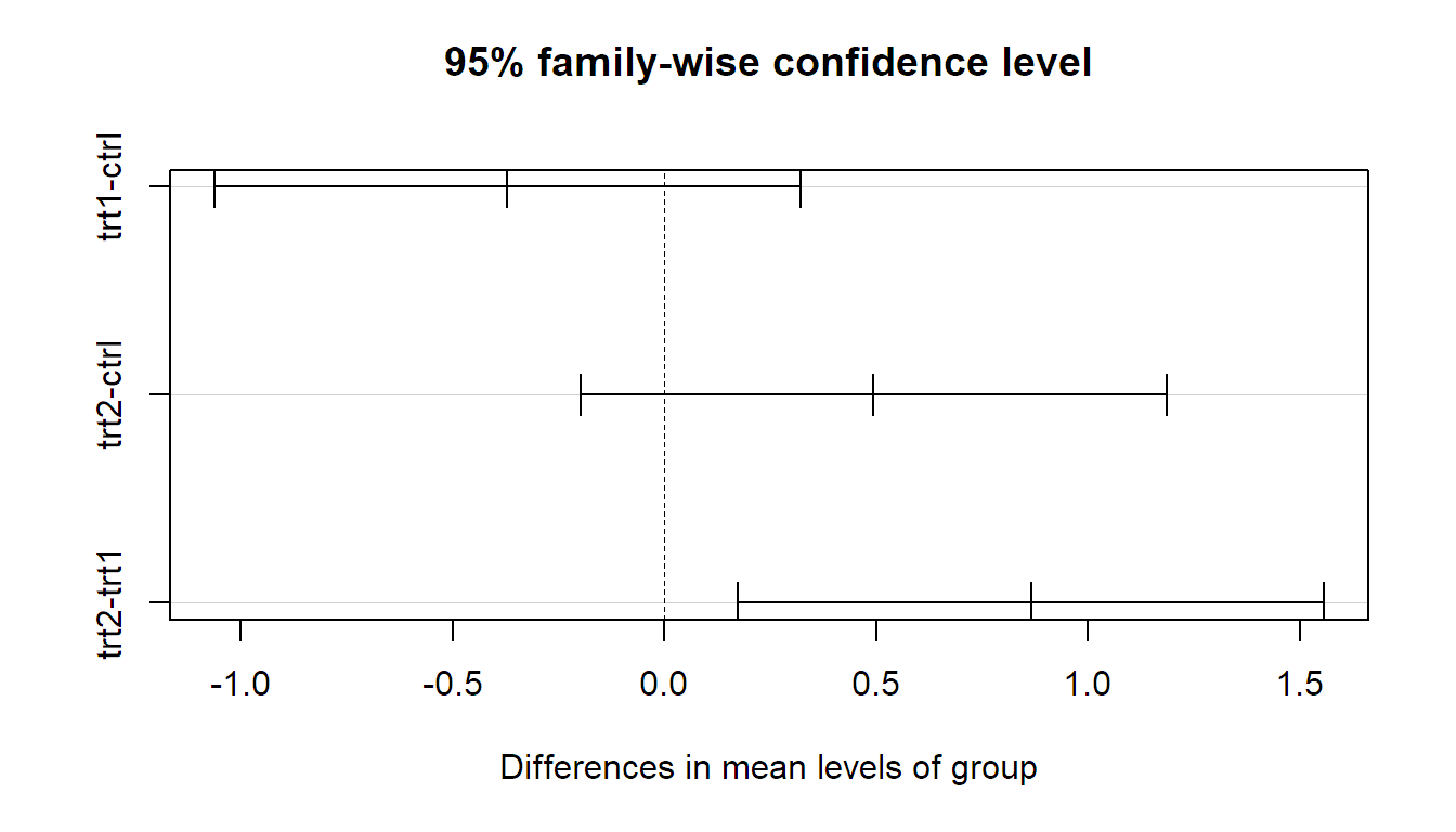
Remember, these confidence intervals are simultaneous, meaning that the
probability that they all cover the corresponding true difference at the same
time is 95%. From the p-values, or the confidence intervals, we read off that only the
difference between trt1 and trt2 is significant (using a significance level
of 5%).
We get of course the same results when using package multcomp. To
do so, we have to use the argument group = "Tukey".
## Tukey HSD with package multcomp
plant.glht.tukey <- glht(fit.plant, linfct = mcp(group = "Tukey"))
summary(plant.glht.tukey)
##
## Simultaneous Tests for General Linear Hypotheses
##
## Multiple Comparisons of Means: Tukey Contrasts
## ...
## Linear Hypotheses:
## Estimate Std. Error t value Pr(>|t|)
## trt1 - ctrl == 0 -0.371 0.279 -1.33 0.391
## trt2 - ctrl == 0 0.494 0.279 1.77 0.198
## trt2 - trt1 == 0 0.865 0.279 3.10 0.012
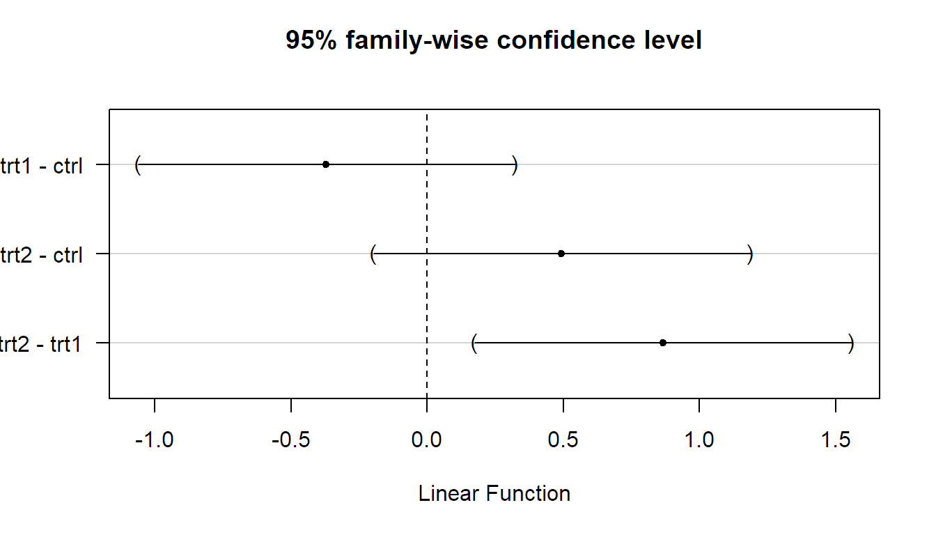
## (Adjusted p values reported -- single-step method)Simultaneous confidence intervals can be obtained by calling confint.
confint(plant.glht.tukey)##
## Simultaneous Confidence Intervals
##
## Multiple Comparisons of Means: Tukey Contrasts
## ...
## 95% family-wise confidence level
## ...
## Linear Hypotheses:
## Estimate lwr upr
## trt1 - ctrl == 0 -0.371 -1.062 0.320
## trt2 - ctrl == 0 0.494 -0.197 1.185
## trt2 - trt1 == 0 0.865 0.174 1.556They can be plotted too.
In emmeans, the corresponding function call would be as follows (output not
shown):
contrast(plant.emm, method = "pairwise")Also with emmeans, the corresponding simultaneous confidence intervals can be
obtained with confint, which can be plotted too.
Remark: The implementations in multcomp and emmeans are more flexible with
respect to unbalanced data than TukeyHSD, especially for situations where we
have multiple factors as for example in Chapter
4.
3.2.5 Multiple Comparisons with a Control
Similarly, if we want to compare all treatment groups with a control
group, we have a so-called multiple comparisons with a control
(MCC) problem (we are basically only
considering a subset of all pairwise comparisons). The corresponding
custom-tailored procedure is called Dunnett procedure (Dunnett 1955). It controls the family-wise error rate in the strong
sense and produces simultaneous confidence intervals. As usual, both
packages multcomp and emmeans provide implementations. By default, the first
level of the factor is taken as the control group. For the factor group in the
PlantGrowth data set this is ctrl, as can be seen when calling the function
levels.
levels(PlantGrowth[,"group"])## [1] "ctrl" "trt1" "trt2"With multcomp, we simply set group = "Dunnett".
##
##   Simultaneous Tests for General Linear Hypotheses
##
## Multiple Comparisons of Means: Dunnett Contrasts
## ...
## Linear Hypotheses:
##                  Estimate Std. Error t value Pr(>|t|)
## trt1 - ctrl == 0   -0.371      0.279   -1.33     0.32
## trt2 - ctrl == 0    0.494      0.279    1.77     0.15
## (Adjusted p values reported -- single-step method)
We get smaller p-values than with the Tukey HSD procedure because we have to correct for less tests; there are more comparisons between pairs than there are comparisons to the control treatment.
In emmeans, the corresponding function call would be as follows (output not
shown):
contrast(plant.emm, method = "dunnett")The usual approach with confint gives the corresponding simultaneous
confidence intervals.
3.2.6 FAQ
Should I only do tests like Tukey HSD, etc. if the \(F\)-test is significant?
No, the above-mentioned procedures have a built-in correction regarding multiple testing and do not rely on a significant \(F\)-test; one exception is the Scheffé procedure in Section 3.2.3: If the \(F\)-test is not significant, you cannot find a significant contrast. In general, conditioning on the \(F\)-test leads to a very conservative approach regarding type I error rate. In addition, the conditional coverage rates of, e.g., Tukey HSD confidence intervals can be very low if we only apply them when the \(F\)-test is significant, see also Hsu (1996). This means that if researchers would use this recipe of only using Tukey HSD when the \(F\)-test is significant and we consider 100 different applications of Tukey HSD, on average it would happen more than 5 times that the simultaneous 95% confidence intervals would not cover all true parameters. Generally speaking, if you apply a statistical test only after a first test was significant, you are typically walking on thin ice: Many properties of the second statistical tests typically change. This problem is also known under the name of selective inference, see for example Benjamini, Heller, and Yekutieli (2009).
Is it possible that the \(F\)-test is significant but Tukey HSD yields only insignificant pairwise tests? Or the other way round, Tukey HSD yields a significant difference but the \(F\)-test is not significant?
Yes, these two tests might give us contradicting results. However, for most situations, this does not happen, see a comparison of the corresponding rejection regions in Hsu (1996).
How can we explain this behavior? This is basically a question of power. For some alternatives, Tukey HSD has more power because it answers a more precise research question, “which pairs of treatments differ?”. On the other hand, the \(F\)-test is more flexible for situations where the effect is not evident in treatment pairs but in combinations of multiple treatments. Basically, the \(F\)-test answers the question, “is a linear contrast of the cell means different from zero?”.
We use the following two extreme data sets consisting of three groups having two observations each.
x <- factor(rep(c("A", "B", "C"), each = 2))

y1 <- c(0.50, 0.62,
        0.46, 0.63,
        0.95, 0.86)

y2 <- c(0.23, 0.34,
        0.45, 0.55,
        0.55, 0.66)
Let us first visualize the first data set:
stripchart(y1 ~ x, vertical = TRUE, pch = 1)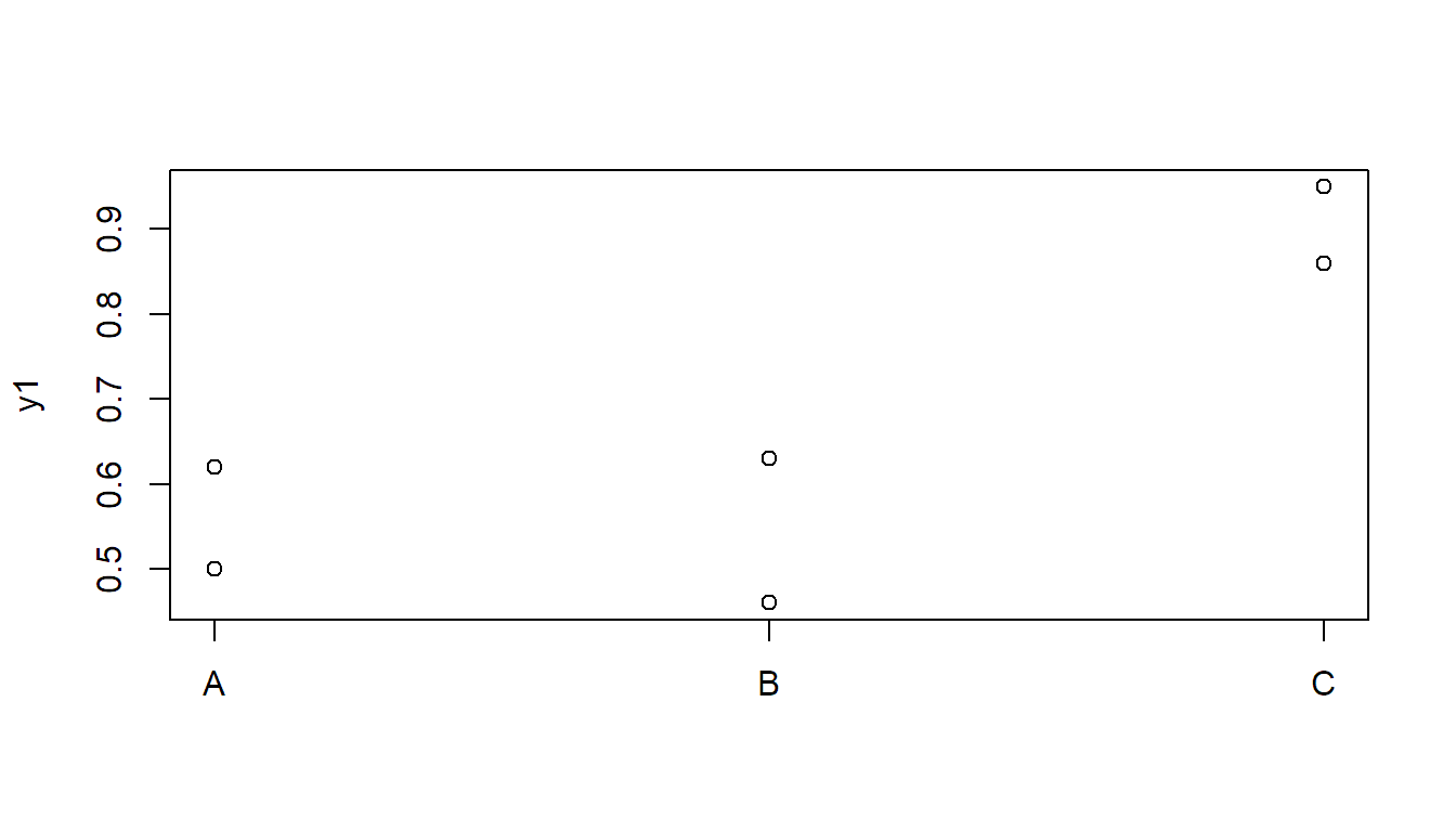
Here, the \(F\)-test is significant, but Tukey HSD is not:
##             Df Sum Sq Mean Sq F value Pr(>F)
## x            2 0.1659  0.0829    9.68  0.049
## Residuals    3 0.0257  0.0086
TukeyHSD(fit1)## Tukey multiple comparisons of means
## 95% family-wise confidence level
## ...
## diff lwr upr p adj
## B-A -0.015 -0.40177 0.3718 0.9857
## C-A 0.345 -0.04177 0.7318 0.0669
## C-B 0.360 -0.02677 0.7468 0.0601Now let us consider the second data set:
stripchart(y2 ~ x, vertical = TRUE, pch = 1)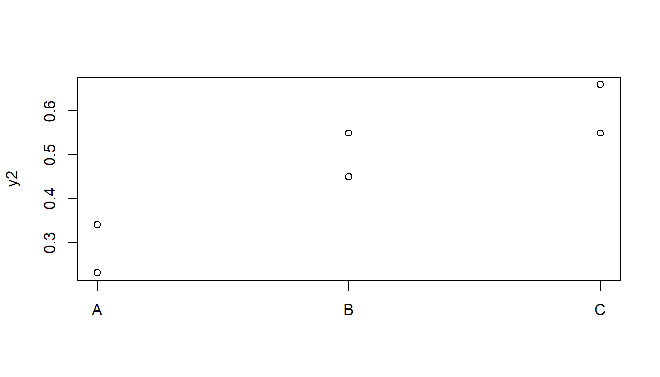
Now, the \(F\)-test is not significant, but Tukey HSD is:
##             Df Sum Sq Mean Sq F value Pr(>F)
## x            2 0.1064  0.0532    9.34  0.052
## Residuals    3 0.0171  0.0057
TukeyHSD(fit2)## Tukey multiple comparisons of means
## 95% family-wise confidence level
## ...
## diff lwr upr p adj
## B-A 0.215 -0.10049 0.5305 0.1269
## C-A 0.320 0.00451 0.6355 0.0482
## C-B 0.105 -0.21049 0.4205 0.4479