sensible summary statistics for big data
The goal of wodds is to make the calculations of whisker
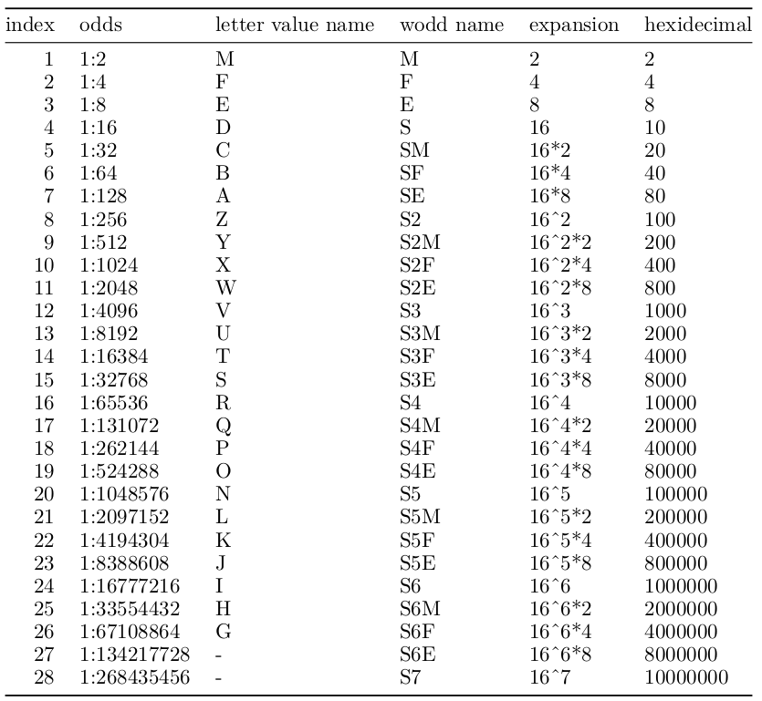
odds (wodds) easy. Wodds follow the same rules as letter-values, but
with a different naming system.
You can install the development version of wodds from GitHub with:
# install.packages("devtools")
devtools::install_github("alexhallam/wodds")This is a basic example which shows you how to solve a common problem:
options(digits=1)
library(wodds)
library(knitr)
set.seed(42)
a <- rnorm(n = 1e4, 0, 1)
df_wodds <- wodds::wodds(a)
df_wodds
#> # A tibble: 11 × 3
#>    lower_value wodd_name upper_value
#>          <dbl> <chr>           <dbl>
#>  1    -0.00625 M            -0.00625
#>  2    -0.694   F             0.663
#>  3    -1.17    E             1.16
#>  4    -1.57    S             1.52
#>  5    -1.88    SM            1.87
#>  6    -2.17    SF            2.15
#>  7    -2.41    SE            2.41
#>  8    -2.66    S2            2.64
#>  9    -2.86    S2M           2.88
#> 10    -3.01    S2F           3.22
#> 11    -3.13    S2E           3.34
Outliers beyond the last wodd are marked with
O<value> in ascending order. There should rarely be
more than 7 outliers when using wodds.
df_wodds_and_outs <- wodds::wodds(a, include_outliers = TRUE)
df_wodds_and_outs
#> # A tibble: 17 × 3
#>    lower_value wodd_name upper_value
#>          <dbl> <chr>           <dbl>
#>  1    -0.00625 M            -0.00625
#>  2    -0.694   F             0.663
#>  3    -1.17    E             1.16
#>  4    -1.57    S             1.52
#>  5    -1.88    SM            1.87
#>  6    -2.17    SF            2.15
#>  7    -2.41    SE            2.41
#>  8    -2.66    S2            2.64
#>  9    -2.86    S2M           2.88
#> 10    -3.01    S2F           3.22
#> 11    -3.13    S2E           3.34
#> 12    -3.14    O1            3.34
#> 13    -3.18    O2            3.47
#> 14    -3.20    O3            3.50
#> 15    -3.33    O4            3.58
#> 16    -3.37    O5            4.33
#> 17    -4.04    O6           NA
Though not necessary it is possible to include tail area if
additional communication or teaching is needed. It is assumed that the
wodd should be explanatory enough to not need to rely on
tail_area.
df_wodds_and_outs <- wodds::wodds(a, include_tail_area  = TRUE)
df_wodds_and_outs
#> # A tibble: 11 × 4
#>    tail_area lower_value wodd_name upper_value
#>        <dbl>       <dbl> <chr>           <dbl>
#>  1         2    -0.00625 M            -0.00625
#>  2         4    -0.694   F             0.663
#>  3         8    -1.17    E             1.16
#>  4        16    -1.57    S             1.52
#>  5        32    -1.88    SM            1.87
#>  6        64    -2.17    SF            2.15
#>  7       128    -2.41    SE            2.41
#>  8       256    -2.66    S2            2.64
#>  9       512    -2.86    S2M           2.88
#> 10      1024    -3.01    S2F           3.22
#> 11      2048    -3.13    S2E           3.34
An example with all options set to TRUE.
df_wodds_and_outs <- wodds::wodds(a, include_depth = TRUE, include_tail_area = TRUE, include_outliers = TRUE)
df_wodds_and_outs
#> # A tibble: 17 × 5
#>    depth tail_area lower_value wodd_name upper_value
#>    <int>     <dbl>       <dbl> <chr>           <dbl>
#>  1     1         2    -0.00625 M            -0.00625
#>  2     2         4    -0.694   F             0.663
#>  3     3         8    -1.17    E             1.16
#>  4     4        16    -1.57    S             1.52
#>  5     5        32    -1.88    SM            1.87
#>  6     6        64    -2.17    SF            2.15
#>  7     7       128    -2.41    SE            2.41
#>  8     8       256    -2.66    S2            2.64
#>  9     9       512    -2.86    S2M           2.88
#> 10    10      1024    -3.01    S2F           3.22
#> 11    11      2048    -3.13    S2E           3.34
#> 12    NA        NA    -3.14    O1            3.34
#> 13    NA        NA    -3.18    O2            3.47
#> 14    NA        NA    -3.20    O3            3.50
#> 15    NA        NA    -3.33    O4            3.58
#> 16    NA        NA    -3.37    O5            4.33
#> 17    NA        NA    -4.04    O6           NA
A knitr::kable example for publication.
knitr::kable(df_wodds_and_outs, align = 'c',digits = 3)| depth | tail_area | lower_value | wodd_name | upper_value |
|---|---|---|---|---|
| 1 | 2 | -0.006 | M | -0.006 |
| 2 | 4 | -0.694 | F | 0.663 |
| 3 | 8 | -1.169 | E | 1.155 |
| 4 | 16 | -1.569 | S | 1.524 |
| 5 | 32 | -1.878 | SM | 1.866 |
| 6 | 64 | -2.173 | SF | 2.150 |
| 7 | 128 | -2.415 | SE | 2.409 |
| 8 | 256 | -2.656 | S2 | 2.637 |
| 9 | 512 | -2.857 | S2M | 2.883 |
| 10 | 1024 | -3.013 | S2F | 3.220 |
| 11 | 2048 | -3.130 | S2E | 3.338 |
| NA | NA | -3.139 | O1 | 3.339 |
| NA | NA | -3.181 | O2 | 3.471 |
| NA | NA | -3.200 | O3 | 3.495 |
| NA | NA | -3.331 | O4 | 3.585 |
| NA | NA | -3.372 | O5 | 4.328 |
| NA | NA | -4.043 | O6 | NA |
wodds::get_depth_from_n(n=15734L, alpha = 0.05)
#> [1] 11wodds::get_n_from_depth(d = 11L)
#> [1] 15734Letter-Values are a fantastic tool! I think the naming could be improved. For this reason I introduce whisker odds (wodds) as an alternative naming system. My hypothesis is that with an alternative naming system the use of these descriptive statistics will be see more use. This is a rebranding of a what I think is a powerful modern statistical tool.