This package provides functions to compute sparse eigenvectors (while keeping their orthogonality) or sparse PCA from either the covariance matrix or directly the data matrix.
# Installation from GitHub
# install.packages("devtools")
devtools::install_github("dppalomar/sparseEigen")

# Get help
library(sparseEigen)
help(package="sparseEigen")
?spEigenspEigen()We start by loading the package and generating synthetic data with sparse eigenvectors:
library(sparseEigen)
set.seed(42)

# parameters
m <- 500  # dimension
n <- 100  # number of samples
q <- 3  # number of sparse eigenvectors to be estimated
sp_card <- 0.1*m  # cardinality of each sparse eigenvector

# generate non-overlapping sparse eigenvectors
V <- matrix(0, m, q)
V[cbind(seq(1, q*sp_card), rep(1:q, each = sp_card))] <- 1/sqrt(sp_card)
V <- cbind(V, matrix(rnorm(m*(m-q)), m, m-q))
# keep first q eigenvectors the same (already orthogonal) and orthogonalize the rest
V <- qr.Q(qr(V))

# generate eigenvalues
lmd <- c(100*seq(from = q, to = 1), rep(1, m-q))

# generate covariance matrix from sparse eigenvectors and eigenvalues
R <- V %*% diag(lmd) %*% t(V)

# generate data matrix from a zero-mean multivariate Gaussian distribution
# with the constructed covariance matrix
X <- MASS::mvrnorm(n, rep(0, m), R)  # random data with underlying sparse structure
Then, we estimate the covariance matrix with cov(X) and
compute its sparse eigenvectors:
# computation of sparse eigenvectors
res_standard <- eigen(cov(X))
res_sparse <- spEigen(cov(X), q)
We can assess how good the estimated eigenvectors are by computing the inner product with the original eigenvectors (the closer to 1 the better):
# show inner product between estimated eigenvectors and originals
abs(diag(t(res_standard$vectors) %*% V[, 1:q])) #for standard estimated eigenvectors
#> [1] 0.9215392 0.9194898 0.9740871
abs(diag(t(res_sparse$vectors) %*% V[, 1:q])) #for sparse estimated eigenvectors
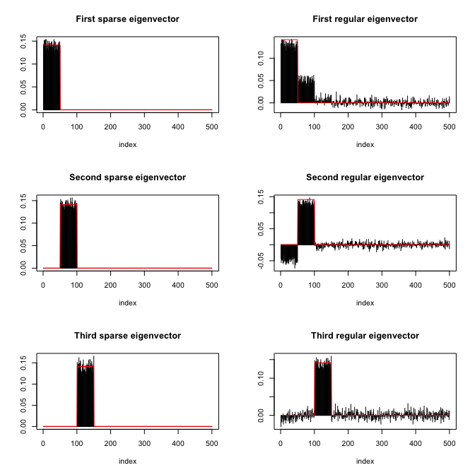
#> [1] 0.9986937 0.9988146 0.9972078Finally, the following plot shows the sparsity pattern of the
eigenvectors (sparse computation vs. classical computation):
spEigenCov()The function spEigenCov() requires more samples than the
dimension (otherwise some regularization is required). Therefore, we
generate data as previously with the only difference that we set the
number of samples to be n=600.
Then, we compute the covariance matrix through the joint estimation of sparse eigenvectors and eigenvalues:
# computation of covariance matrix
res_sparse2 <- spEigenCov(cov(X), q)
Again, we can assess how good the estimated eigenvectors are by computing the inner product with the original eigenvectors:
# show inner product between estimated eigenvectors and originals
abs(diag(t(res_sparse2$vectors[, 1:q]) %*% V[, 1:q]))    #for sparse estimated eigenvectors
#> [1] 0.9997197 0.9996029 0.9992848
Finally, we can compute the error of the estimated covariance matrix (sparse eigenvector computation vs. classical computation):
# show error between estimated and true covariance
norm(cov(X) - R, type = 'F') #for sample covariance matrix
#> [1] 48.42514
norm(res_sparse2$cov - R, type = 'F') #for covariance with sparse eigenvectors
#> [1] 25.74865