The goal of smoots is to provide an easy way to estimate
the nonparametric trend and its derivatives in trend-stationary,
equidistant time series with short-memory stationary errors. The main
functions allow for data-driven estimates via local polynomial
regression with an automatically selected optimal bandwidth.
You can install the released version of smoots from CRAN with:
install.packages("smoots")This is a basic example which shows you how to solve a common
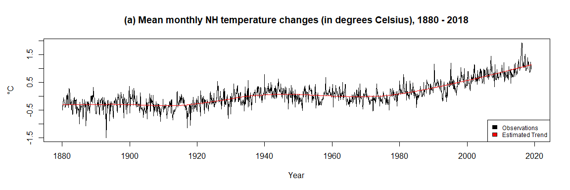
problem. The data tempNH in the package includes the mean
monthly temperature changes in degrees Celsius of the Northern
Hemisphere (NH) from 1880 to 2018. The data was obtained from the
Goddard Institute for Space Studies of the National Aeronautics and
Space Administration (NASA). To make use of the smoots
package, it has to be assumed that the data follows an additive model
consisting of a deterministic, nonparametric trend function and a
zero-mean stationary rest with short-range dependence.
The user-friendly and simply applicable function
msmooth() for the estimation of trend function in the
additive model will be used.
library(smoots) # Call the packagedata <- tempNH # Call the 'tempNH' data frame
Yt <- data$Change # Store the actual values as a vector
# Estimate the trend function via the 'smoots' package
results <- msmooth(Yt, p = 1, mu = 1, bStart = 0.15, alg = "A")
# Easily access the main estimation results
b.opt <- results$b0 # The optimal bandwidth
trend <- results$ye # The trend estimates
resid <- results$res # The residuals
b.opt
#> [1] 0.101089
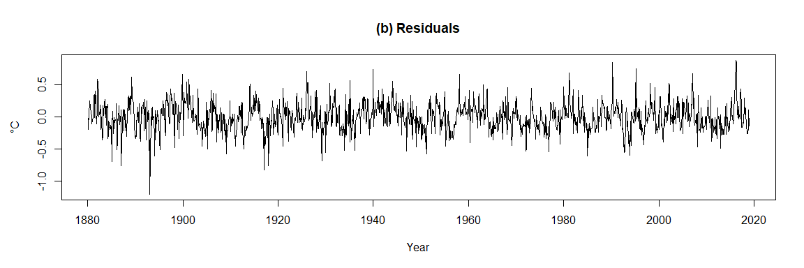
An optimal bandwidth of 0.101089 was selected by the iterative
plug-in algorithm (IPI) within msmooth(). Moreover, the
estimated trend fits the data suitably and the residuals seem to be
stationary. Since the trend was obtained without any parametric
assumptions with respect to the rest term, the detrended values could
now be further analyzed by means of any suitable parametric approach,
e.g. autoregressive-moving-average (ARMA) models.
With the package version 1.1.0 different functions were newly introduced that allow for forecasting trend-stationary series and other functionalities. Based on the previous example, the following code shows how to obtain point forecasts and 95% forecasting intervals for the mean monthly temperature changes data and directly create a plot of the forecasting results. For simplicity, it is assumed that the rest term of the additive model follows an ARMA(1,1) model with normally distributed innovations. However, via the functions a bootstrap method for non-Gaussian cases can be applied as well. Furthermore, an automatic order selection for the ARMA model is also built-in that is triggered, if no values are passed to the respective arguments that define the orders.
n <- length(Yt)
# Create a vector with exact time points (optional for the plot)
time <- seq(from = 1880 + 1 / 12, to = 2019, by = 1 / 12)

# Application of the forecasting function with automatic creation of a graphic
forecast <- modelCast(results, p = 1, q = 1, h = 5, alpha = 0.95,
  method = "norm", plot = TRUE, x = time, type = "b",
  col = "deepskyblue4", pch = 20, lty = 2,
  main = "Title (series is cut-off)",
  xlab = "Exemplary x-axis label", ylab = "Exemplary y-axis label")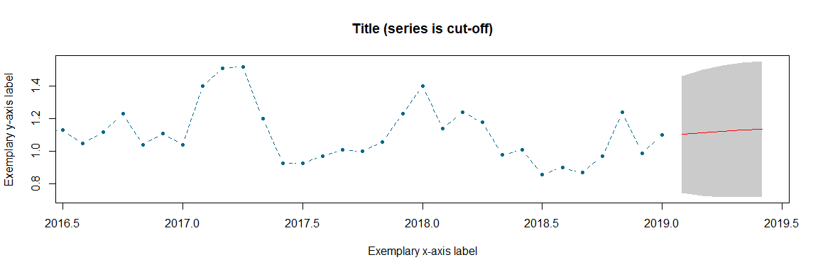
forecast
#>             k=1       k=2       k=3       k=4       k=5
#> fcast 1.1041137 1.1151230 1.1240264 1.1313490 1.1374849
#> 2.5%  0.7468131 0.7281308 0.7212654 0.7199682 0.7213253
#> 97.5% 1.4614144 1.5021152 1.5267873 1.5427297 1.5536445Another contribution that was made to package version 1.1.0 is a function for testing the trend graphically for linearity. Based on a previously obtained nonparametric estimate of the trend or its derivatives, an asymptotically unbiased series of estimates with its confidence bounds is obtained and plotted. By choice, different polynomial regression lines can be displayed alongside the nonparametric trend estimates and its confidence bounds. The estimated slope of a simple linear regression model of the trend and the constant with value zero are displayed against the estimates of the first and second derivatives, respectively. If, for a selected confidence level 100s%, clearly more than (1 - s)100% of the estimated parametric line lies outside of the confidence bounds, the null hypothesis can be rejected. The following example is based yet again on the mean monthly temperature changes data and illustrates the linearity test with respect to the nonparametric trend. The derivatives are skipped at this point for simplicity. Moreover, a confidence level of 95% was chosen.
# Calculation of confidence bounds with creation of a graphic
bounds <- confBounds(results, alpha = 0.95, p = 1, x = time)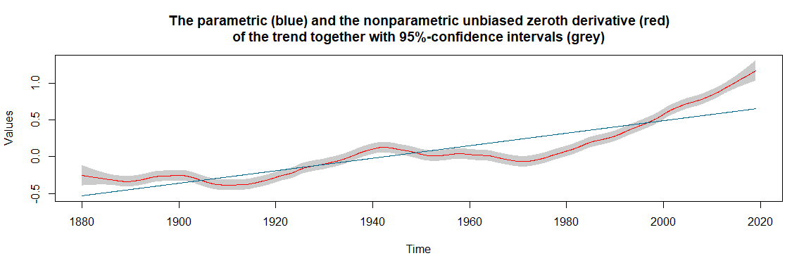
bounds
#> -----------------------------------------------
#> | Results of the confidence bounds estimation |
#> -----------------------------------------------
#>
#> Number of observations:   1668
#> Order of derivative:         0
#> Adjusted bandwidth:     0.0570
For the (asymptotically) unbiased estimation of the trend function an adjusted bandwidth of 0.057 was used. Since more than 5% of the linear regression line (blue) lies outside of the grey confidence bounds, we can reject the null hypothesis that the trend is linear.
The trend estimation functions can also be used for the
implementation of semiparametric generalized autoregressive conditional
heteroskedasticity (Semi-GARCH) models and its various variants in
Financial Econometrics (see also the examples in the documentation of
msmooth() and tsmooth()).
In smoots fourteen functions are available.
Original functions since version 1.0.0:
dsmooth: Data-driven Local Polynomial for the Trend’s
Derivatives in Equidistant Time Seriesgsmooth: Estimation of Trends and their Derivatives via
Local Polynomial Regressionknsmooth: Estimation of Nonparametric Trend Functions
via Kernel Regressionmsmooth: Data-driven Nonparametric Regression for the
Trend in Equidistant Time Seriestsmooth: Advanced Data-driven Nonparametric Regression
for the Trend in Equidistant Time SeriesNewly introduced with version 1.1.0:
rescale: Rescaling Derivative EstimatescritMatrix: ARMA Order Selection MatrixoptOrd: Optimal Order SelectionnormCast: Forecasting Function for ARMA Models under
Normally Distributed InnovationsbootCast: Forecasting Function for ARMA Models via
BootstraptrendCast: Forecasting Function for Nonparametric Trend
FunctionsmodelCast: Forecasting Function for Trend-Stationary
Time SeriesrollCast: Backtesting Semi-ARMA Models with Rolling
ForecastsconfBounds: Asymptotically Unbiased Confidence
BoundsFor further information on each of the functions, we refer the user to the manual or the package documentation.