![]()
SEMinR allows users to easily create and modify structural equation models (SEM). It allows estimation using either covariance-based SEM (CBSEM, such as LISREL/Lavaan), or Partial Least Squares Path Modeling (PLS-PM, such as SmartPLS/semPLS).
Main features of using SEMinR:
Take a look at the easy syntax and modular design:
# Define measurements with famliar terms: reflective, composite, multi-item constructs, etc.
measurements <- constructs(
  reflective("Image",       multi_items("IMAG", 1:5)),
  composite("Expectation", multi_items("CUEX", 1:3)),
  composite("Loyalty",     multi_items("CUSL", 1:3), weights = mode_B),
  composite("Complaints",  single_item("CUSCO"))
)

# Create four relationships (two regressions) in one line!
structure <- relationships(
  paths(from = c("Image", "Expectation"), to = c("Complaints", "Loyalty"))
)

# Estimate the model using PLS estimation scheme (Consistent PLS for reflectives)
pls_model <- estimate_pls(data = mobi, measurements, structure)
#> Generating the seminr model
#> All 250 observations are valid.

# Re-estimate the model as a purely reflective model using CBSEM
cbsem_model <- estimate_cbsem(data = mobi, as.reflective(measurements), structure)
#> Generating the seminr model for CBSEM
SEMinR can plot models using the semplot (for CBSEM models) or
DiagrammeR (for PLS models) packages with a simple plot
method.
plot(pls_model, title = "PLS Model")
save_plot("myfigure.pdf")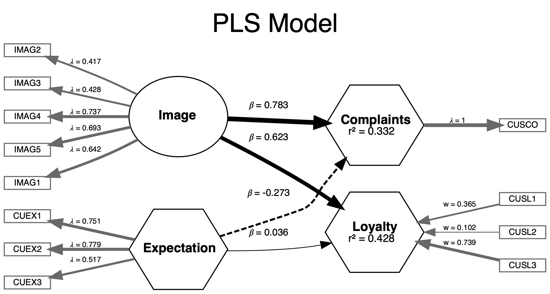
SEMinR allows various estimation methods for constructs and SEMs:
Researchers can now create a SEM and estimate it using different techniques (CBSEM, PLS-PM).
You can install SEMinR from R with:
install.packages("seminr")Load the SEMinR package:
library(seminr)Describe measurement and structural models and then estimate them. See the various examples below for different use cases:
Note that CBSEM models reflective common-factor constructs, not composites. SEMinR uses the powerful Lavaan package to estimate CBSEM models – you can even inspect the more complicated Lavaan syntax that is produced.
Describe reflective constructs and interactions:
# Distinguish and mix composite or reflective (common-factor) measurement models
# - composite measurements will have to be converted into reflective ones for CBSEM (see below)
measurements <- constructs(
  reflective("Image",       multi_items("IMAG", 1:5)),
  reflective("Expectation", multi_items("CUEX", 1:3)),
  interaction_term(iv = "Image", moderator = "Expectation", method = two_stage),
  reflective("Loyalty",     multi_items("CUSL", 1:3)),
  reflective("Complaints",  single_item("CUSCO"))
)
Describe the causal relationships between constructs and interactions:
# Quickly create multiple paths "from" and "to" sets of constructs
structure <- relationships(
  paths(from = c("Image", "Expectation", "Image*Expectation"), to = "Loyalty"),
  paths(from = "Image", to = c("Complaints"))
)
Put the above elements together to estimate the model using Lavaan:
# Evaluate only the measurement model using Confirmatory Factor Analysis (CFA)
cfa_model <- estimate_cfa(data = mobi, measurements)
summary(cfa_model)

# Dynamically compose full SEM models from individual parts
# - if measurement model includes composites, convert all constructs to reflective using:
#     as.reflective(measurements)
cbsem_model <- estimate_cbsem(data = mobi, measurements, structure)
sum_cbsem_model <- summary(cbsem_model)
sum_cbsem_model$meta$syntax # See the Lavaan syntax if you wishModels with reflective common-factor constructs can also be estimated in PLS-PM, using Consistent-PLS (PLSc). Note that the popular SmartPLS software models constructs as composites rather than common-factors (see below) but can also do PLSc as a special option.
We will reuse the measurement and structural models from earlier:
# Optionally inspect the measuremnt and structural models
measurements
structure
Estimate full model using Consistent-PLS and bootstrap it for confidence intervals:
# Models with reflective constructs are automatically estimated using PLSc
pls_model <- estimate_pls(data = mobi, measurements, structure)
summary(pls_model)

# Use multi-core parallel processing to speed up bootstraps
boot_estimates <- bootstrap_model(pls_model, nboot = 1000, cores = 2)
summary(boot_estimates)
PLS-PM typically models composites (constructs that are weighted average of items) rather than common factors. Popular software like SmartPLS models composites either as Mode A (correlation weights) or Mode B (regression weights). We also support both modes as well as second-order composites. rather than common factors. Popular software like SmartPLS models composites by default, either as Mode A (correlation weights) or Mode B (regression weights). We also support second-order composites.
Describe measurement model for each composite, interaction, or higher order composite:
# Composites are Mode A (correlation) weighted by default
mobi_mm <- constructs(
  composite("Image",        multi_items("IMAG", 1:5)),
  composite("Value",        multi_items("PERV", 1:2)),
  higher_composite("Satisfaction", dimensions = c("Image","Value"), method = two_stage),
  composite("Expectation",  multi_items("CUEX", 1:3)),
  composite("Quality",      multi_items("PERQ", 1:7), weights = mode_B),
  composite("Complaints",   single_item("CUSCO")),
  composite("Loyalty",      multi_items("CUSL", 1:3), weights = mode_B)
)
Define a structural (inner) model for our PLS-PM:
mobi_sm <- relationships(
  paths(from = c("Expectation","Quality"),  to = "Satisfaction"),
  paths(from = "Satisfaction", to = c("Complaints", "Loyalty"))
)
Estimate full model using PLS-PM and bootstrap it for confidence intervals:
pls_model <- estimate_pls(
  data = mobi,
  measurement_model = mobi_mm,
  structural_model = mobi_sm
)

summary(pls_model)

# Use multi-core parallel processing to speed up bootstraps
boot_estimates <- bootstrap_model(pls_model, nboot = 1000, cores = 2)
summary(boot_estimates)SEMinR can plot all supported models using the dot language and the
graphViz.js widget from the DiagrammeR package.
# generate a small model for creating the plot
mobi_mm <- constructs(
  composite("Image",        multi_items("IMAG", 1:3)),
  composite("Value",        multi_items("PERV", 1:2)),
  higher_composite("Satisfaction", dimensions = c("Image","Value"), method = two_stage),
  composite("Quality",      multi_items("PERQ", 1:3), weights = mode_B),
  composite("Complaints",   single_item("CUSCO")),
  reflective("Loyalty",      multi_items("CUSL", 1:3))
)
mobi_sm <- relationships(
  paths(from = c("Quality"),  to = "Satisfaction"),
  paths(from = "Satisfaction", to = c("Complaints", "Loyalty"))
)
pls_model <- estimate_pls(
  data = mobi,
  measurement_model = mobi_mm,
  structural_model = mobi_sm
)
#> Generating the seminr model
#> Generating the seminr model
#> All 250 observations are valid.
#> All 250 observations are valid.
boot_estimates <- bootstrap_model(pls_model, nboot = 100, cores = 1)
#> Bootstrapping model using seminr...
#> SEMinR Model successfully bootstrapped
When we have a model, we can plot it and save the plot to files.
plot(boot_estimates, title = "Bootstrapped Model")
save_plot("myfigure.pdf")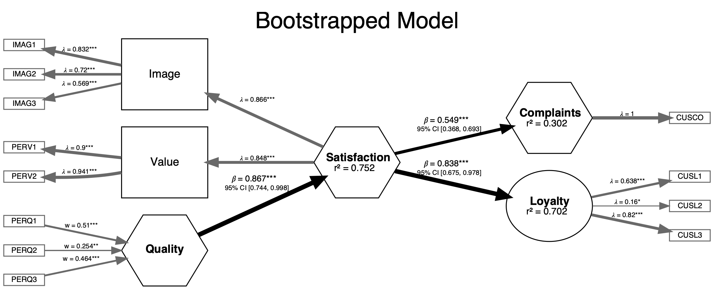
We can customize the plot using an elaborate theme. Themes can be
used for individual plots as a parameter or set as a default. Using the
seminr_theme_create() function allows to define different
themes.
# Tip: auto complete is your friend in finding all possible themeing options.
thm <- seminr_theme_create(plot.rounding = 2, plot.adj = FALSE,
                           sm.node.fill = "cadetblue1",
                           mm.node.fill = "lightgray")
# change new default theme - valid until R is restarted
seminr_theme_set(thm)

# the new plot
plot(boot_estimates)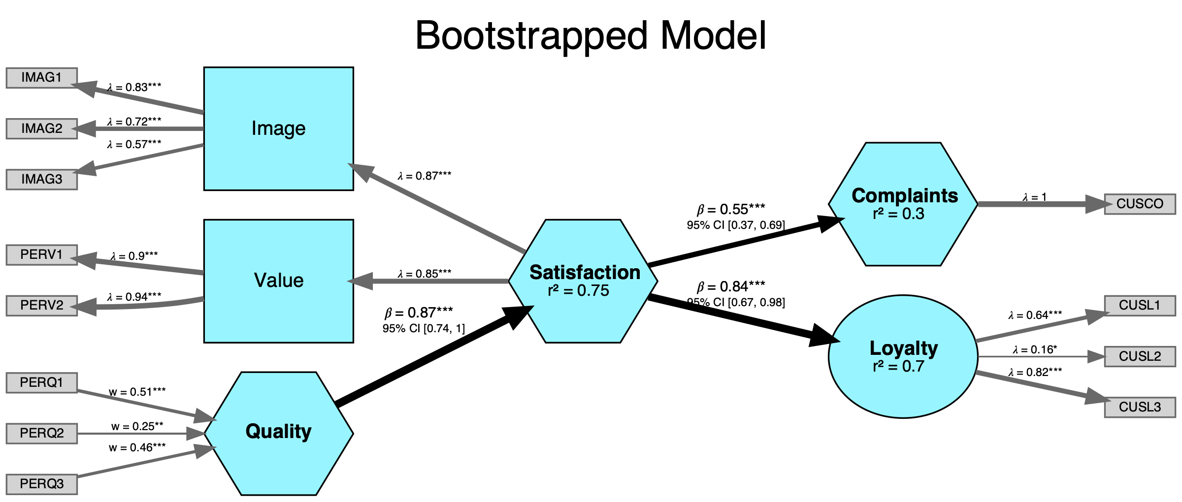
We can re-estimate a composite PLS-PM model as a common-factor CBSEM. Such a comparison might interest researchers seeking to evaluate how their constructs behave when modeled as composites versus common-factors.
# Define measurements with famliar terms: reflective, multi-item constructs, etc.
measurements <- constructs(
  composite("Image",       multi_items("IMAG", 1:5)),
  composite("Expectation", multi_items("CUEX", 1:3)),
  composite("Loyalty",     multi_items("CUSL", 1:3)),
  composite("Complaints",  single_item("CUSCO"))
)

# Create four relationships (two regressions) in one line!
structure <- relationships(
  paths(from = c("Image", "Expectation"), to = c("Complaints", "Loyalty"))
)

# First, estimate the model using PLS
pls_model <- estimate_pls(data = mobi, measurements, structure)

# Reusable parts of the model to estimate CBSEM results
# note: we are using the `as.reflective()` function to convert composites to common factors
cbsem_model <- estimate_cbsem(data = mobi, as.reflective(measurements), structure)

# Re-estimate the model using common factors in Consistent PLS (PLSc)
pls_model <- estimate_pls(data = mobi, as.reflective(measurements), structure)The vignette for Seminr can be found on GitHub or by running the
vignette("SEMinR") command after installation.
Demo code for various use cases with SEMinR can be
found in the seminr/demo/
folder or by running commands such as
demo("seminr-contained") after installation.
Model Specification:
Model Visualization:
Syntax Style:
We communicate and collaborate with several other open-source projects on SEM related issues.
Facebook Group: https://www.facebook.com/groups/seminr
You will find the developers and other users here who might also be able to help or discuss.
Issue Tracker: https://github.com/sem-in-r/seminr/issues
This is the official place to submit potential bugs or request new features for consideration.
Primary Authors:
Key Contributors:
And many thanks to the growing number of folks who have reached out with feature requests, bug reports, and encouragement. You keep us going!