prism
![]()
This package allows users to access and visualize data from the Oregon State PRISM project. Data are all in the form of gridded rasters for the continental US at 4 different temporal scales: daily, monthly, annual, and 30 year normals. Please see their webpage for a full description of the data products, or see their overview.
prism is available on CRAN:
install.packages("prism")Or the development version can be installed from GitHub with devtools:
# install.packages("devtools")
library(devtools)
install_github("ropensci/prism")The overall work flow in the prism package is (links go to details on this page):
prism_set_dl_dir(). This is now referred to as the “prism
archive”.get_prism_*(). Each folder, or variable,
timestep, day/month/year is stored in a single folder in the archive and
referred to as prism data (pd).prism_archive_*(). Or interact with
the prism data: pd_*().The remainder of this README provides examples following this work flow.
Data are available in 4 different temporal scales as mentioned above. At each temporal scale, there are 11 different parameters/variables available. Keep in mind these are modeled parameters, not measured. Please see the full description for how they are calculated.
| Parameter name | Description |
|---|---|
| tmean | Mean temperature |
| tmax | Maximum temperature |
| tmin | Minimum temperature |
| tdmean | Mean dew point temperature |
| ppt | Total precipitation (rain and snow) |
| vpdmin | Daily minimum vapor pressure deficit |
| vpdmax | Daily maximum vapor pressure deficit |
| solclear | Solar radiation (clear sky) |
| solslope | Solar radiation (sloped) |
| soltotal | Solar radiation (total) |
| soltrans | Cloud transmittance |
Normals (4km or 800m resolution) based on 1991-2020 average:
Important .bil
files are no longer available in .bil format. The
get_prism_normals() functions still work and will download
the data in GeoTiff format. But - the rest of the prism
R package has not been updated to work with GeoTiff, so none of the
other functions will work with the 30-year normal data, e.g.,
prism_archive_subset(temp_period = "monthly normals") will
return character(0) and plotting functions will not
work.
| Variable | Annual | Monthly | Daily |
|---|---|---|---|
| tmean | X | X | X |
| tmax | X | X | X |
| tmin | X | X | X |
| tdmean | X | X | X |
| ppt | X | X | X |
| vpdmin | X | X | X |
| vpdmax | X | X | X |
| solclear | 800m | 800m | |
| solslope | 800m | 800m | |
| soltotal | 800m | 800m | |
| soltrans | 800m | 800m |
Daily, monthly, and annual data:
| Variable | Annual (1895-present) | Monthly (1895-present) | Daily (1981-present) |
|---|---|---|---|
| tmean | X | X | X |
| tmax | X | X | X |
| tmin | X | X | X |
| tdmean | X | X | X |
| ppt | X | X | X |
| vpdmin | X | X | X |
| vpdmax | X | X | X |
| solclear | |||
| solslope | |||
| soltotal | |||
| soltrans |
Before downloading any data, set the directory that the prism data will be saved to:
library(prism)
#> Be sure to set the download folder using `prism_set_dl_dir()`.
prism_set_dl_dir("~/prismtmp")
This is now referred to as the “prism archive”. The
prism_archive_*() functions allow the user to search
through the archive. The prism archive contains “prism data”. The prism
data are referred to by their folder names, even though the “real” data
are the .bil, .txt, and other files that exist in the folder. The prism
data (pd) can be accessed using the pd_*()
functions.
Normals are based on the latest 30-year period; currently 1991 - 2020. Normals can be downloaded in two resolutions, 4km and 800m, and a resolution must be specified. They can be downloaded for a given day, month, vector of days/months, or annual averages for all 30 years.
# Download March 14 30-year average precip. Note the year is ignored
get_prism_normals('ppt', '4km', day = as.Date('2025-03-14'))

# Download the January - June 30-year averages at 4km resolution
get_prism_normals(type="tmean", resolution = "4km", mon = 1:6, keepZip = FALSE)

# Download the 30-year annual average precip and annual average temperature
get_prism_normals("ppt", "4km", annual = TRUE, keepZip = FALSE)
get_prism_normals("tmean", "4km", annual = TRUE, keepZip = FALSE)
If the archive has not already been set, calling any of the
get_prism_*() functions will prompt the user to specify the
directory. prism data are downloaded as zip files and then unzipped. If
the keepZip argument is TRUE the zip file will
remain on your machine, otherwise it will be automatically deleted.
Let us download daily average temperatures from June 1 to June 14, 2013. We can also download January average temperature data from 1982 to 2014. Finally, we will download annual average precipitation for 2000 to 2015. Note that resolution must now be specified for all data downloads.
get_prism_dailys(
  type = "tmean",
  minDate = "2013-06-01",
  maxDate = "2013-06-14",
  resolution = "4km",
  keepZip = FALSE
)
get_prism_monthlys(
  type = "tmean",
  years = 1982:2014,
  mon = 1,
  resolution = "4km",
  keepZip = FALSE
)
get_prism_annual(
  type = "ppt",
  years = 2000:2015,
  resolution = "4km",
  keepZip = FALSE
)
Note that for daily data you need to give a well formed date string in the form of “YYYY-MM-DD”.
You can view all the prism data you have downloaded with a simple
command: prism_archive_ls(). This function gives a list of
folder names, i.e., prism data (pd). All the functions in
the prism package work off of one or more of these folder names
(pd).
## Truncated to keep file list short
prism_archive_ls()
#>  [1] "prism_ppt_us_25m_191004"
#>  [2] "prism_ppt_us_25m_191401"
#>  [3] "prism_ppt_us_25m_191402"
#>  [4] "prism_ppt_us_25m_191403"
#>  [5] "prism_ppt_us_25m_191404"
#>  [6] "prism_ppt_us_25m_191405"
#>  [7] "prism_ppt_us_25m_191406"
#>  [8] "prism_ppt_us_25m_191407"
#>  [9] "prism_ppt_us_25m_191408"
#> [10] "prism_ppt_us_25m_191409"
....
While prism functions use this folder format, other files may need an
absolute path (e.g. the raster package). The
pd_to_file() function conveniently returns the absolute
path. Alternatively, you may want to see what the normal name for the
product is (not the file name), and we can get that with the
pd_get_name() function.
## Truncated to keep file list short
pd_to_file(prism_archive_ls()[1:10])
#>  [1] "C:\\Users\\RAButler\\Documents\\prismtmp\\prism_ppt_us_25m_191004\\prism_ppt_us_25m_191004.bil"
#>  [2] "C:\\Users\\RAButler\\Documents\\prismtmp\\prism_ppt_us_25m_191401\\prism_ppt_us_25m_191401.bil"
#>  [3] "C:\\Users\\RAButler\\Documents\\prismtmp\\prism_ppt_us_25m_191402\\prism_ppt_us_25m_191402.bil"
#>  [4] "C:\\Users\\RAButler\\Documents\\prismtmp\\prism_ppt_us_25m_191403\\prism_ppt_us_25m_191403.bil"
#>  [5] "C:\\Users\\RAButler\\Documents\\prismtmp\\prism_ppt_us_25m_191404\\prism_ppt_us_25m_191404.bil"
....

pd_get_name(prism_archive_ls()[1:10])
#>  [1] "Apr  1910 - 4km resolution - Precipitation"
#>  [2] "Jan  1914 - 4km resolution - Precipitation"
#>  [3] "Feb  1914 - 4km resolution - Precipitation"
#>  [4] "Mar  1914 - 4km resolution - Precipitation"
#>  [5] "Apr  1914 - 4km resolution - Precipitation"
....
Finally, prism_archive_subset() is a convenient way to
search for specific parameters, time steps, days, months, years, or
ranges of days, months, years. Note that resolution must be
specified for all archive subset operations.
# we know we have downloaded June 2013 daily data, so lets search for those
prism_archive_subset("tmean", "daily", mon = 6, resolution = "4km")
#>  [1] "prism_tmean_us_25m_20130601" "prism_tmean_us_25m_20130602"
#>  [3] "prism_tmean_us_25m_20130603" "prism_tmean_us_25m_20130604"
#>  [5] "prism_tmean_us_25m_20130605" "prism_tmean_us_25m_20130606"
#>  [7] "prism_tmean_us_25m_20130607" "prism_tmean_us_25m_20130608"
#>  [9] "prism_tmean_us_25m_20130609" "prism_tmean_us_25m_20130610"
#> [11] "prism_tmean_us_25m_20130611" "prism_tmean_us_25m_20130612"
#> [13] "prism_tmean_us_25m_20130613" "prism_tmean_us_25m_20130614"

# or we can look for days between June 7 and June 10
prism_archive_subset(
  "tmean", "daily",
  minDate = "2013-06-07",
  maxDate = "2013-06-10",
  resolution = "4km"
)
#> [1] "prism_tmean_us_25m_20130607" "prism_tmean_us_25m_20130608"
#> [3] "prism_tmean_us_25m_20130609" "prism_tmean_us_25m_20130610"You can easily make a quick plot of your data using the output of
prism_archive_ls() or prism_archive_subset()
with pd_image().
# Plot the precipitation in 2000
ppt2002 <- prism_archive_subset(
  "ppt", "annual", year = 2002, resolution = "4km"
)
pd_image(ppt2002)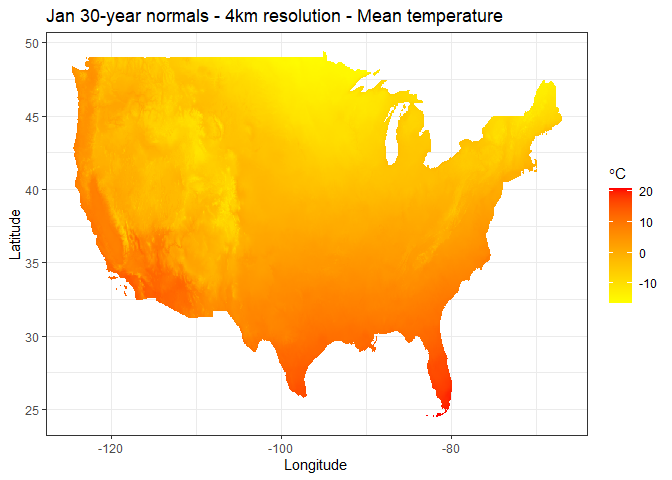
It is easy to load the prism data with the raster package. This time we will look at the difference in precipitation between 2011 and 2002. Conveniently, we already downloaded these data. We just need to grab them out of our archive.
library(raster)
#> Warning: package 'raster' was built under R version 4.5.1
#> Loading required package: sp
#> Warning: package 'sp' was built under R version 4.5.1
# knowing the name of the files you are after allows you to find them in the
# list of all files that exist
# ppt2002 <- "prism_ppt_us_25m_2002"
# ppt2011 <- "prism_ppt_us_25m_2011"
# but we will use prism_archive_subset() to find the files we need

ppt2002_name <- prism_archive_subset(
  "ppt", "annual", year = 2002, resolution = "4km"
)
ppt2011_name <- prism_archive_subset(
  "ppt", "annual", year = 2011, resolution = "4km"
)

# raster needs a full path, not the "short" prism data name
ppt2002 <- pd_to_file(ppt2002_name)
ppt2011 <- pd_to_file(ppt2011_name)

## Now we'll load the rasters.
ppt2002_rast <- raster(ppt2002)
ppt2011_rast <- raster(ppt2011)

# Now we can do simple subtraction to get the anomaly by subtracting 2014
# from the 30 year normal map
diff_calc <- function(x, y) {
  return(x - y)
}

anom_rast <- raster::overlay(ppt2002_rast, ppt2011_rast, fun = diff_calc)

plot(anom_rast)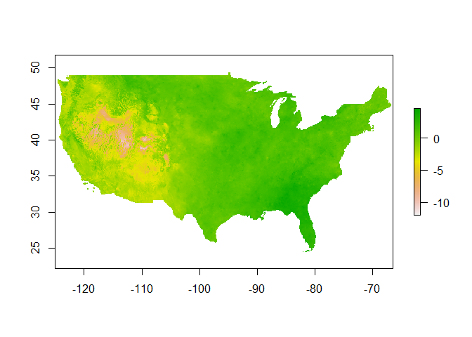
The plot shows which regions were wetter in 2011 than 2002 (and the reverse). It also shows how easy it is to use the raster library to work with prism data. The package provides a simple framework to work with a large number of rasters that you can easily download and visualize or use with other data sets.
You can also visualize a single point across multiple prism data
files (slice) using pd_plot_slice(). This procedure will
take a set of rasters, create a “raster::stack”, extract
data at a point, and then create a ggplot2 object.
Let’s now make a plot of January temperatures in Boulder between 1982
and 2014. First we’ll grab all the data from the US (downloaded in the
previous step), and then give our function a point to get data from. The
point must be a vector in the form of longitude, latitude. Because
pd_plot_slice() returns a gg object, it can be combined
with other ggplot functions.
library(ggplot2)
#> Warning: package 'ggplot2' was built under R version 4.5.1
# data already exist in the prism dl dir
boulder <- c(-105.2797, 40.0176)

# prism_archive_subset() will return prism data that matches the specified
# variable, time step, years, months, days, etc.
to_slice <- prism_archive_subset("tmean", "monthly", mon = 1, resolution = "4km")
p <- pd_plot_slice(to_slice, boulder)

# add a linear average and title
p +
  stat_smooth(method="lm", se = FALSE) +
  theme_bw() +
  ggtitle("Average January temperature in Boulder, CO 1982-2014")
#> `geom_smooth()` using formula = 'y ~ x'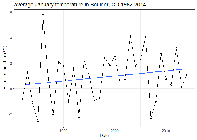
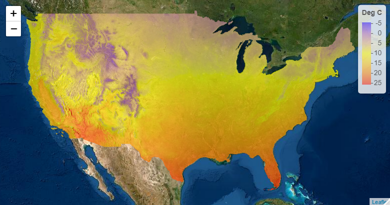
Finally, the prism data are in a form that can be used with leaflet maps (with the help of the raster package). The leaflet package allows you to easily make JavaScript maps using the leaflet mapping framework using prism data. These can easily be hosted on websites like Rpubs or your own site. Here is a simple example of plotting the 30-year normal for annual temperature. If you run this code you will have an interactive map, instead of just the screen shot shown here.
library(leaflet)
library(raster)
library(prism)

# January 2002 average temperature has already been downloaded
norm <- prism_archive_subset(
  "tmean", "monthly", mon = 1, year = 2002, resolution = "4km"
)
rast <- raster(pd_to_file(norm))

# Create color palette and plot
pal <- colorNumeric(
  c("#0000FF", "#FFFF00", "#FF0000"),
  values(rast),
  na.color = "transparent"
)

leaflet() %>%
  addTiles(
    urlTemplate = 'http://server.arcgisonline.com/ArcGIS/rest/services/World_Imagery/MapServer/tile/{z}/{y}/{x}'
  ) %>%
  addRasterImage(rast, colors = pal, opacity=.65) %>%
  addLegend(pal = pal, values = values(rast), title = "Deg C")
[