plantTracker
plantTracker
![]()
![]()
![]()
![]()
Welcome to plantTracker! This package was designed to
transform long-term quadrat maps that show plant
occurrence and size into demographic data that can be
used to answer questions about population and community ecology.
plantTrackerplantTracker
Install plantTracker from CRAN:
install.packages("plantTracker")Alternatively, you can install the current version of
plantTracker from GitHub:
install.packages("devtools")
devtools::install_github("aestears/plantTracker")Please report any problems that you encounter while using
plantTracker as “issues” on (our GitHub repository)[https://github.com/aestears/plantTracker/issues/]. Help
us make this package better!
This package is licensed under MIT License Copyright (c) 2022 Alice Stears
Questions about plantTracker can be forwarded to Alice
Stears, the package maintainer, at
alice.e.stears@gmail.com.
Follow this link to a shiny app that lets you change arguments in the trackSpp() function, and see how that impacts individual ID assignment in an example dataset: https://astears.shinyapps.io/shinyapp/
plantTracker R packageThe material below explains how to use plantTracker,
starting with formatting your data correctly. This information is also
available in the ‘Suggested plantTracker Workflow’
vignette, which is included in the package.
The functions in plantTracker require data in a specific
format. plantTracker includes an example dataset that
consists of two pieces: grasslandData and
grasslandInventory. You can load these example datasets
into your global environment by calling data(grasslandData)
and data(grasslandInventory). You can view the
documentation for these datasets by calling?grasslandData
and ?grasslandInventory.
Most plantTracker functions require two data objects.
The first is a data frame that contains the location and metadata for
each mapped individual, which we from now on will call dat.
The second is a list that contains a vector of years in which each
quadrat was sampled, which we from now on will cal inv.
Below are the basic requirements for these data objects.
dat
data frame must . . .sf data.frame. More on this below in section 1.1.1…sf package data format) that contains a polygon
representing the location of each observation. Each observation must be
a POLYGON or MULTIPOLYGON. Data cannot be
stored as POINTS.dat does not need to have a coordinate reference system
(i.e. CRS can be “NA”), but it can have one if you’d like.plantTracker functions.plantTracker functions.Here are the first few rows of a possible dat input
data.frame:
#> Simple feature collection with 6 features and 6 fields
#> Geometry type: POLYGON
#> Dimension:     XY
#> Bounding box:  xmin: -0.000160084 ymin: 0.4334812 xmax: 0.286985 ymax: 0.9419673
#> CRS:           NA
#>                 Species Type Site Quad Year sp_code_6
#> 1 Heteropogon contortus poly   AZ  SG2 1922    HETCON
#> 2 Heteropogon contortus poly   AZ  SG2 1922    HETCON
#> 3 Heteropogon contortus poly   AZ  SG2 1922    HETCON
#> 4 Heteropogon contortus poly   AZ  SG2 1922    HETCON
#> 5 Heteropogon contortus poly   AZ  SG2 1922    HETCON
#> 6 Heteropogon contortus poly   AZ  SG2 1922    HETCON
#>                         geometry
#> 1 POLYGON ((0.237747 0.908835...
#> 2 POLYGON ((0.2833037 0.85959...
#> 3 POLYGON ((0.008583123 0.449...
#> 4 POLYGON ((0.1480142 0.46983...
#> 5 POLYGON ((0.03573306 0.5259...
#> 6 POLYGON ((0.2441894 0.52689...plantTracker functions.Here’s what some of the example dat data (from the “SG2”
quadrat at the “AZ” site in 1922) look like when plotted spatially:
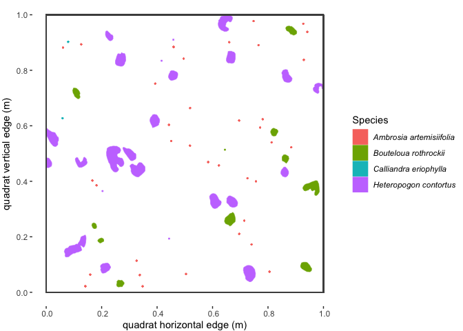
Figure 1.1 : Spatial map of a subset of example ‘dat’ dataset
It’s important to note that, while plantTracker was
designed to be used with small-scale maps of plant occurrence in
quadrats, it is conceivably possible to use other styles of map data in
plantTracker functions. All that is required is a single
mapped basal area (or point location converted to a small polygon) at
each time point for each organism (or ramet), and is accompanied by the
required metadata detailed above. For example, plantTracker
functions could be used to estimate tree demographic rates at the scale
of 100 m x 50 m plots.
sf data formatAs mentioned above, plantTracker uses the
sf R package to deal with spatial data. The map data that
plantTracker was built to analyze is inherently spatial, so
you need to know how to the basics of dealing with spatial data in R if
you want to use plantTracker! There are many good resources
to help you orient yourself to working with spatial data in R
generally:
And the sf package more specifically:
These resources provide a great orientation, and while I recommend
looking over them if you’re new to working with spatial data in R, I’ve
included a brief tutorial for uploading shapefiles into R as
sf data frames.
Most of the published chart-quadrat datasets have the map data stored
as shapefiles in complex file structures, which can be a bit confusing
to navigate. plantTracker requires all of your data (for
all species, plots and years) to be in one single data frame. This
example shows how you might navigate through a complex file structure to
to pull out shapefiles and put them into one single sf data
frame. for further analysis with plantTracker. For
this example, I’ll use a subset of the data from the Santa Rita
Experimental Range in Arizona, which has been published in this
data paper. In this dataset, shapefiles for each quadrat are stored
in their own folder. Within that folder there are two shapefiles for
each year: one that contains map data for polygons, and one that
contains data for points. The following code reads in those shapefiles,
transforms the points to polygons of a fixed radius, and puts all the
data into one sf data frame. If you want to follow along,
download the “shapefiles.zip” file from the data paper, un-zip it, and
name it “AZ_shapefiles”. The dataset that is the result of this example
is the same as part of the “grasslandData” dataset included in
plantTracker.
#  save a character vector of the file names in the file that contains the
# shapefiles (in this case, called "CO_shapefiles"), each of which is a quadrat
# note: 'wdName' is a character string indicating the path of the directory
# containing the 'AZ_shapefiles' folder
quadNames <- list.files(paste0(wdName,"AZ_shapefiles/"))
# trim the quadrats down to 2, for the sake of runtime in this example
quadNames <- quadNames[quadNames %in% c("SG2", "SG4")]

# now we'll loop through the quadrat folders to download the data
for (i in 1:2){#length(quadNames)) {
  # get the names of the quadrat for this iteration of the loop
  quadNow <- quadNames[i]
  #  get a character vector of the unique quad/Year combinations of data in
  # this folder that contain polygon data
  quadYears <- quadYears <-  unlist(strsplit(list.files(
    paste0(wdName, "AZ_shapefiles/",quadNow,"/"),
    pattern = ".shp$"), split = ".shp"))
  # loop through each of the years in this quadrat
  for (j in 1:length(quadYears)) {
    # save the name of this quadYear combo
    quadYearNow <- quadYears[j]
    # read in the shapefile for this quad/year combo as an sf data frame
    # using the 'st_read()' function from the sf package
    shapeNow <- sf::st_read(dsn = paste0(wdName,"AZ_shapefiles/",quadNow),
                            #  the 'dsn' argument is the folder that
                            # contains the shapefile files--in this case,
                            # the folder for this quadrat
                            layer = quadYearNow) # the 'layer' argument has the
    # name of the shapefile, without the filetype extension! This is because each
    # shapefile consists of at least three separate files, each of which has a
    # unique filetype extension.
    # the shapefiles in this dataset do not have all of the metadata we
    # need, and have some we don't need, so we'll remove what we don't need and
    # add columns for 'site', 'quad', and 'year'
    shapeNow$Site <- "AZs"
    shapeNow$Quad <- quadNow
    # get the Year for the shapefile name--in this case it is the last for
    # numbers of the name
    shapeNow$Year <- as.numeric(strsplit(quadYearNow, split = "_")[[1]][2]) + 1900
    # determine if the 'current' quad/year contains point data or polygon data
    if (grepl(quadYearNow, pattern = "C")) { # if quadYearNow has point data
      # remove the columns we don't need
      shapeNow <- shapeNow[,!(names(shapeNow)
                              %in% c("Clone", "Seedling", "Area", "Length", "X", "Y"))]
      # reformat the point into a a very small polygon
      # (a circle w/ a radius of .003 m)
      shapeNow <- sf::st_buffer(x = shapeNow, dist = .003)
      # add a column indicating that this observation was originally
      # mapped as a point
      shapeNow$type <- "point"
    } else { # if quadYearNow has polygon data
      # remove the columns we don't need
      shapeNow <- shapeNow[,!(names(shapeNow) %in% c("Seedling", "Canopy_cov", "X", "Y", "area"))]
      # add a column indicating that this observation was originally
      # mapped as a polygon
      shapeNow$type <- "polygon"
    }
    # now we'll save this sf data frame
    if (i == 1 & j == 1) { # if this is the first year in the first quadrat
      dat <- shapeNow
    } else { # if this isn't the first year in the first quadrat, simply rbind
      # the shapeNow sf data frame onto the previous data
      dat <- rbind(dat, shapeNow)
    }
  }
}

# Now, all of the spatial data are in one sf data frame!
# for the sake of this example, we'll remove data for some species and years in order to make the example run faster (and to make this 'dat' data.frame identical to the "grasslandData" dataset included in this R pakcage).
dat <- dat[dat$Species %in% c("Heteropogon contortus", "Bouteloua rothrockii", "Ambrosia artemisiifolia", "Calliandra eriophylla", "Bouteloua gracilis", "Hesperostipa comata", "Sphaeralcea coccinea", "Allium textile"),]
dat <- dat[  (dat$Quad %in% c("SG2", "SG4") &
             dat$Year %in% c(1922:1927)),]
In some spatial datasets, observations that were measured as “points”
in the field are still stored as “points” in the shapefiles.
plantTracker requires all observations to be stored as
“polygon” geometry in order to streamline functions, so we need to
translate “points” into small polygons of a fixed area. In this case,
we’ll transform them into circles with a radius of 1 cm (.01, since this
dataset measures area in meters). ‘dat’ has a column called “type.” A
value of “point” in this column will tell us that, even though the
geometry of the “point” data is now in “polygon” format, the values for
basal area and growth are not indicative of the true size of the
plant.
# We use the function "st_buffer()" to add a buffer of our chosen radius (.01) around each point observation, which will transform each observation into a circle of the "polygon" format with a radius of .01.
dat_1 <- st_buffer(x = dat[st_is(x = dat, type = "POINT"),], dist = .01)
dat_2 <- dat[!st_is(x = dat, type = "POINT"),]
dat <- rbind(dat_1, dat_2)
If you don’t want to download the data and format it into an sf data.frame, you can also use a subset of the “grasslandData” data object stored in this R package. You will just need to subset it to include only the data from the “AZ” site. Code to do this is below:
dat <- grasslandData[grasslandData$Site == "AZ",]inv list
must . . .dat. There cannot be two elements
with the same name, and there cannot be an element with more than one
quadrat in its name. There must be an element for each quadrat with data
in dat.dat
(i.e. if year is a four-digit number in dat, then it must
be a four-digit number in inv). Make sure this is the years
the quadrat was actually sampled, not just the years that have data in
the dat data frame! This argument allows the function to
differentiate between years when the quadrat wasn’t sampled and years
when there just weren’t any individuals of a species present in that
quadrat. If a quadrat wasn’t sampled in a given year, don’t put an ‘NA’
in inv for that year! Instead, just skip that year.Here is an example of an inv argument that corresponds
to the example dat argument above. The quadrats that have
data in dat are “SG2” and “SG4”, so there are elements in
inv that correspond to each of these quadrats.
#> $SG2
#> [1] 1922 1923 1924 1925 1926 1927
#>
#> $SG4
#> [1] 1922 1923 1924 1925 1926 1927
If you already have a quadrat inventory as a data frame, it isn’t
complicated to reformat it to work with plantTracker
functions. For example, if your quadrat inventory data frame looks like
this… :
#>   quad1 quad2 quad3
#> 1  2000  2000  2000
#> 2  2001  2001    NA
#> 3    NA  2002  2002
#> 4  2003  2003  2003
#> 5  2004  2004  2004
#> 6  2005  2005  2005
#> 7  2006  2006  2006
#> 8  2007  2007  2007
… then do the following to get it into a format ready for
plantTracker:
quadInv_DF <- data.frame("quad1" = c(2000, 2001, NA, 2003, 2004, 2005, 2006, 2007),
           "quad2" = c(2000:2007),
           "quad3" = c(2000, NA, 2002, 2003, 2004, 2005, 2006, 2007))

# use the 'as.list()' function to transform your data frame into a named list
quadInv_list <- as.list(quadInv_DF)
# we still need to remove the 'NA' values, which we can do using the
# 'lapply()' function
(quadInv_list <- lapply(X = quadInv_list, FUN = function(x) x[is.na(x) == FALSE]))
#> $quad1
#> [1] 2000 2001 2003 2004 2005 2006 2007
#>
#> $quad2
#> [1] 2000 2001 2002 2003 2004 2005 2006 2007
#>
#> $quad3
#> [1] 2000 2002 2003 2004 2005 2006 2007inv and dat arguments using
checkDat()The generic checkDat() function:
checkDat(dat, inv = NULL, species = "Species", site = "Site", quad = "Quad",
  year = "Year", geometry = "geometry", reformatDat = FALSE, ...)
This step is optional, but can be useful if you’re unsure whether
your dat and inv arguments are in the correct
format. The plantTracker function checkDat()
takes dat and inv as arguments for the
arguments dat andinv, and will return
informative error messages if either argument is not in the correct
format.
Additional optional arguments to checkDat() are
species, site, quad,
year, geometry, and
reformatDat.
species/site/quad/year/geometry
These arguments only need to be included if the columns in
dat that contain the data for species, site, quadrat, year
and geometry of each observation are different from the names
“Species”, “Site”, “Quad”, “Year, and”geometry”. For example, if the
column in your version of dat that contains the species
identity of each observation is called “species_names”, then the
argument species = "species_names" must be included in your
call to checkDat().
reformatDat is a TRUE/FALSE
argument that determines whether you want the checkDat()
function to return a version of dat that is ready to go
into the steps of this workflow. If reformatDat = TRUE then
checkDat() will return a list that contains the reformatted
version of dat, the reformatted version of inv
and an additional element called “userColNames”, which contains the
column names in the input version of dat that are different
from the expected column names of “Species”, “Site”, “Quad”, “Year,
and”geometry” (if there are any). If reformatDat = TRUE,
then checkDat() will return a message indicating that your
data is ready for the next step. The default value is FALSE.
trackSpp()Now it’s time to transform your raw dataset into demographic data!
This is accomplished using the trackSpp() function. This
function follows individual plants from year to year in the same quadrat
to determine survival, size in the next year, age, and some additional
potentially-useful demographic data. It does this by comparing quadrat
maps from sequential years. If there is overlap of individuals of the
same species in consecutive years, then the rows in dat
that contain data for those overlapping individuals are given the same
“trackID”, or unique identifier.
Here is the generic trackSpp() function:
trackSpp(dat, inv, dorm, buff, buffGenet, clonal, species = "Species",
  site = "Site", quad = "Quad", year = "Year", geometry = "geometry",
  aggByGenet = TRUE, printMessages = TRUE, flagSuspects = FALSE,
shrink = 0.1, dormSize = 0.05, ...)trackSpp() takes the following arguments:
dat This is the sf data
frame that we’ve been calling dat so far. This must be in
the correct format (which you can check before-hand using
checkDat()), but informative error messages will be
returned if it is incorrect. It must have the columns outlined
in Section 1.1, but they can have different
names as long as those names are included in this function call (more on
that later…).inv This is the list of quadrat
sampling years we’ve been calling inv. If it is not in the
correct format or does not contain data for the correct quadrats, then
an informative error message will be returned.dorm This is a positive integer value
that indicates how long you want the function to allow an individual to
be “dormant”. In this case, dormancy can be interpreted as the
biological phenomenon where a plant has above-ground tissue present in
year 1, is alive underground but with no above-ground tissue in year 2,
and then has above-ground tissue in a subsequent year. Dormancy can also
be interpreted here as data-collection error, whereby an individual is
accidentally not mapped in between years where it was recorded.Consider the following example: There is a polygon of
species “A” in year 1, which is our “focal individual”. In year 2, there
is not a polygon of species “A” that overlaps with our focal individual.
In year 3, there is a polygon of species “A” that is in the same
location as our focal individual. If dorm = 0, then our
focal individual would get a 0 in the survival column, and the polygon
of species “A” in year 3 would be considered a new recruit and get a new
trackID. If dorm = 1, because there is overlap between two
polygons of the same species with only a 1-year gap between when they
occur, these two polygons will be considered the same genetic
individual, will have the same trackID, and our focal individual will
have a “1” in the survival column. In an alternative scenario, in years
3 and 4 there are not polygons of species “A” that are in the same
location as our focal individual, but there is a polygon in year 4 that
overlaps our focal individual. If dorm = 1, then our focal
individual would get a “0” for survival, but if dorm = 2,
then it would get a 1 for survival.
#> Warning: Using `size` aesthetic for lines was deprecated in ggplot2 3.4.0.
#> ℹ Please use `linewidth` instead.
#> This warning is displayed once every 8 hours.
#> Call `lifecycle::last_lifecycle_warnings()` to see where this warning was
#> generated.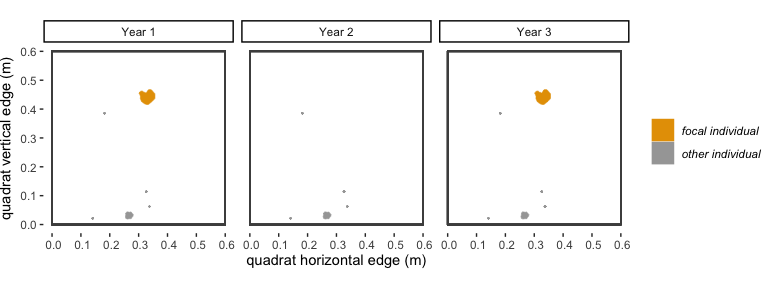
Figure 2.1: A visualization of the ‘dormancy’ scenario described above.
If you’d like to be more specific and perhaps biologically accurate,
you can also specify the dorm argument uniquely for each
species. For example, it might be that you are confident that your data
collectors did not accidentally “miss” any individuals, and your
dat data frame contains observations for shrubs or trees,
which are very unlikely to go dormant, and small forbs, which are much
more likely to go dormant for one or two years. In order to disallow
dormancy for trees and shrubs, but to allow dormancy for forbs, you will
provide a data frame to the dorm argument instead of a
single positive integer value. There will be two columns: 1) a “Species”
column that has the species name for each species present in
dat, and 2) a column called “dorm” that has positive
integer values indicating the dormancy you’d like to allow for each
species. Make sure that if you are following the data frame approach,
you must provide a dormancy argument for every species that has
data in dat. Make sure that the species names in the
dorm data frame are spelled exactly the same as they are in
dat. The data frame should look something like this:
#>   Species dorm
#> 1  tree A    0
#> 2 shrub B    0
#> 3  tree C    0
#> 4  forb D    1
#> 5  forb E    2
#> 6  forb F    1
Important Note: Be very careful about how you define the
dorm argument. The bigger the dorm argument,
the more likely you are to overestimate survival. For annually-sampled
data, I would need a very biologically-compelling reason to to specify a
dorm argument greater than 1 year.
buff This is a positive numeric
value that indicates how much an individual can move from year 1 to year
2 and still be considered the same individual (receive the same
trackID). In addition to accounting for true variation in location of a
plant’s stem from year to year, this argument also accounts for small
inconsistencies in mapping from year to year. The buff
argument must be in the same units as the spatial values in
dat. For example, if the spatial data in dat
is measured in meters, and you want to allow a plant to “move” 15 cm
between year 1 and year 2, then you would include the argument
buff = .15 in your call to trackSpp(). If you
want to allow no movement, use buff = 0. Below is a
visualization of two different buff scenarios.
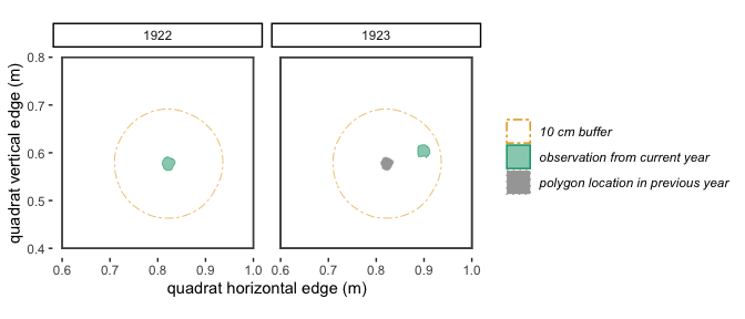
Figure 2.2: With a 10 cm buffer, these polygons in 1922 and 1923 overlap and will be identified by trackSpp() as the same individual and receive the same trackID.
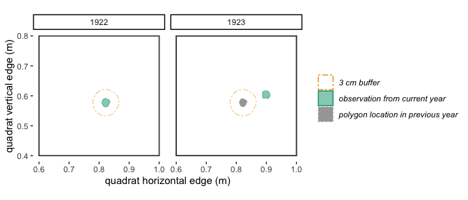
Figure 2.3: With a 3 cm buffer, these polygons in 1922 and 1923 don’t quite overlap, so will be identified by trackSpp() as different individuals and receive different trackIDs.
clonal This is a logical argument
(TRUE or FALSE) that indicates whether you want to allow plants to be
clonal or not. In the context of this type of data, “clonal” means that
one genetic individual (or “genet”) can be recorded as multiple polygons
(or “ramets”). If clonal = TRUE, then multiple polygons in
the same year can be part of the same individual and have the same
trackID. If clonal = FALSE, then every polygon in a given
year is a unique individual and has a unique trackID. This option can be
defined globally for all species present in dat by setting
clonal equal to FALSE or TRUE in the
trackSpp() function call. Alternatively,
clonal can be specified uniquely for each species by
creating a data frame that contains a clonal argument for
each species (analogous to the data frame for the dorm
argument shown in Table 2.1, but with a column called “clonal”).The following arguments to trackSpp() are only required
in certain contexts.
buffGenet is an argument that is only
required if clonal = TRUE or if clonal is a
data frame that contains at least a single TRUE in the
“clonal” column. buffGenet is a numeric value that
indicates how close polygons of the same species must be to one another
in the first year in order to be considered parts of the same genetic
individual (ramets of the same genet). Similar to buff, be
very careful and conservative when defining this argument. A large value
for buffGenet can quickly lead to the entire quadrat being
treated as the same genetic individual! I suggest experimenting with
multiple values of buffGenet, looking at maps that show the
trackID assignment, and deciding on a value that leads to trackID
assignments that make the most biological sense to you. This argument is
passed to the groupByGenet() function, which assigns the
same trackID to individuals that are within the buffGenet
buffer of each other. Polygons are only grouped by genet in the first
year of data. After that point, grouping by genet happens based on data
in previous years. If there are multiple polygons that overlap with a
genet in the previous year, they are given the same trackID and are
considered ramets belonging to the same genet. The value of
buffGenet must be greater than or equal to zero, and must
be in the same units as the spatial data in dat.
buffGenet can be a single numeric value which will be
applied to all species present in dat, or can be specified
uniquely for each species by creating a data frame that contains a
buffGenet argument for each species (analogous to the data
frame for the dorm argument shown in Table 2.1, but with a
column called “buffGenet”).aggByGenet is a logical argument that
is only required if clonal = TRUE or if clonal
is a data frame that contains at least a single TRUE in the
“clonal” column. This argument determines whether the output data frame
from trackSpp() will have a row for every single ramet, or
will be aggregated so that each genet is represented by a single row. If
aggByGenet = FALSE, then the output is not aggregated. If
aggByGenet = TRUE (the default setting), then the results
are aggregated using the plantTracker function
aggregateByGenet(). This function combines the
sf “POLYGONS” for each ramet into one sf
MULTIPOLYGON for the entire genet, and combines the
associated metadata (“Species”, “Site”, “Quad”, “Year”, “trackID”,
“basalArea_genet”, “age”, “recruit”, “survives_tplus1”, “size_tplus1”,
“nearEdge”) into one row for this genet. Even if the input
dat had additional columns, they will not be included in
the output of trackSpp if aggByGenet = TRUE,
since it is uncertain if they can be summed across all ramets or are
identical across all ramets. For example, if each ramet has a unique
character string in a column called “name”, there is no easy way to
“sum” the character strings in this column to have one value for each
genet. If you want the output data frame from trackSpp() to
have the same columns as your input dat data.frame, set the
aggByGenet argument to FALSE. However, Be Careful, since
any demographic analysis should be done with a data.set that has only
one row per genet, otherwise you will be estimating survival and growth
rates on the scale of ramets instead of genets. If you take the
aggByGenet = FALSE route, be sure to pass your dataset
through the aggregateByGenet() function (or aggregate to
the genet scale using your preferred method) before demographic
analysis.species/site/quad/year/geometry These
arguments only need to be included if the columns in dat
that contain the data for species, site, quadrat, year and geometry of
each observation are different from the names “Species”,
“Site”, “Quad”, “Year, and”geometry”. For example, if the column in your
version of dat that contains the species identity of each
observation is called “species_names”, then the argument
species = "species_names" must be included in your call to
trackSpp().printMessages This is an optional
logical argument that determines whether this function returns messages
about genet aggregation, as well as messages indicating which year is
the last year of sampling in each quadrat and which year(s) come before
a gap in sampling that exceeds the dorm argument (and thus
which years of data have an “NA” for “survives_tplus1” and
“size_tplus1”). If printMessages = TRUE (the default), then
messages are printed. If printMessages = FALSE, then
messages are not printed.flagSuspects This is an optional
logical argument of length 1, indicating whether observations that are
“suspect” will be flagged. The default
isflagSuspects = FALSE. If
flagSuspects = TRUE, then a column called “Suspect” is
added to the output data.frame. Any suspect observations get a “TRUE” in
the “Suspect” column, while non-suspect observations receive a “FALSE”.
There are two ways that an observation can be classified as “suspect”.
First, if two consecutive observations have the same trackID, but the
observation in year t+1 is less that a certain percentage (defined by
the shrink arg.) of the observation in year t, it is
possible that the observation in year t+1 is a new recruit and not the
same individual. The second way an observation can be classified as
“suspect” is if it is very small before going dormant. It is unlikely
that a very small individual will survive dormancy, so it is possible
that the function has mistakenly given a survival value of “1” to this
individual. A “very small individual” is any observation with an area
below a certain percentile (specified by dormSize) of the
size distribution for this species, which is generated using all of the
size data for this species in dat. If you are using the
output dataset for demographic analysis, you may want to exclude
“Suspect” observations. If flagSuspects = FALSE, then no
additional column is added.shrink This is an optional argument
that takes a single numeric value. This value is only used when
flagSuspects = TRUE. When two consecutive observations have
the same trackID, and the ratio of size_t+1 to size_t is smaller than
the value of shrink, the observation in year t gets a
“TRUE” in the “Suspect” column. For example, shrink = 0.2,
and an individual that the tracking function has identified as
“BOUGRA_1992_5” has an area of 9 cm\(^2\) in year_t and an area of 1.35 cm\(^2\) in year_t+1. The ratio of size_t+1 to
size_t is 1.35/9 = 0.15, which is smaller than the cutoff specified by
shrink, so the observation of “BOUGRA_1992_5” in year t
gets a “TRUE” in the “Suspect” column. The default value is
shrink = 0.10.dormSize This is an optional argument
that takes a single numeric value. This value is only used when
flagSuspects = TRUE and dorm ≥ 1. An
individual is flagged as “suspect” if it “goes dormant” and has a size
that is less than or equal to the percentile of the size distribution
for this species that is designated by dormSize. For
example, dormSize = 0.05, and an individual has a basal
area of 0.5 cm\(^2\). The 5th
percentile of the distribution of size for this species, which is made
using the mean and standard deviation of all observations in
dat for the species in question, is 0.6 cm\(^2\). This individual does not have any
overlaps in the next year (year_t+1), but does have an overlap in
year_t+2. However, because the basal area of this observation is smaller
than the 5th percentile of size for this species, the observation in
year t will get a “TRUE” in the “Suspect” column. It is possible that
the tracking function has mistakenly assigned a “1” for survival in
year_t, because it is unlikely that this individual is large enough to
survive dormancy. The default value is dormSize = .05.These are all of the possible arguments to
trackSpp()!
Below is an example of a potential function call to
trackSpp(), using the example dat and
inv data we’ve used so far. :
datTrackSpp <- plantTracker::trackSpp(dat = dat, inv = inv,
         dorm = 1,
         buff = .05,
         buffGenet = .005,
         clonal = data.frame("Species" = c("Heteropogon contortus",
                                           "Bouteloua rothrockii",
                                           "Ambrosia artemisiifolia",
                                           "Calliandra eriophylla"),
                             "clonal" = c(TRUE,TRUE,FALSE,FALSE)),
         aggByGenet = TRUE,
         printMessages = FALSE
         )
And here’s what the output of this call to trackSpp()
looks like:
#> Simple feature collection with 477 features and 12 fields
#> Geometry type: GEOMETRY
#> Dimension:     XY
#> Bounding box:  xmin: -0.001386579 ymin: -0.001017592 xmax: 1.000536 ymax: 1.001267
#> CRS:           NA
#> First 10 features:
#>    Site Quad                 Species        trackID Year  type    basalArea
#> 1    AZ  SG2 Ambrosia artemisiifolia  AMBART_1922_1 1922 point 2.461883e-05
#> 2    AZ  SG2 Ambrosia artemisiifolia AMBART_1922_10 1922 point 2.461883e-05
#> 3    AZ  SG2 Ambrosia artemisiifolia AMBART_1922_11 1922 point 2.461883e-05
#> 4    AZ  SG2 Ambrosia artemisiifolia AMBART_1922_12 1922 point 2.461883e-05
#> 5    AZ  SG2 Ambrosia artemisiifolia AMBART_1922_13 1922 point 2.461883e-05
#> 6    AZ  SG2 Ambrosia artemisiifolia AMBART_1922_14 1922 point 2.461883e-05
#> 7    AZ  SG2 Ambrosia artemisiifolia AMBART_1922_15 1922 point 2.461883e-05
#> 8    AZ  SG2 Ambrosia artemisiifolia AMBART_1922_16 1922 point 2.461883e-05
#> 9    AZ  SG2 Ambrosia artemisiifolia AMBART_1922_17 1922 point 2.461883e-05
#> 10   AZ  SG2 Ambrosia artemisiifolia AMBART_1922_18 1922 point 2.461883e-05
#>    recruit survives_t+1 age size_t+1 nearEdge                       geometry
#> 1       NA            0  NA       NA     TRUE POLYGON ((0.350604 0.021361...
#> 2       NA            0  NA       NA    FALSE POLYGON ((0.7172048 0.25834...
#> 3       NA            0  NA       NA    FALSE POLYGON ((0.1845598 0.38566...
#> 4       NA            0  NA       NA    FALSE POLYGON ((0.759387 0.399850...
#> 5       NA            0  NA       NA    FALSE POLYGON ((0.1696044 0.40291...
#> 6       NA            0  NA       NA    FALSE POLYGON ((0.7290925 0.41097...
#> 7       NA            0  NA       NA    FALSE POLYGON ((0.6255546 0.45737...
#> 8       NA            0  NA       NA    FALSE POLYGON ((0.5872073 0.46925...
#> 9       NA            0  NA       NA    FALSE POLYGON ((0.8863168 0.52256...
#> 10      NA            0  NA       NA    FALSE POLYGON ((0.5212498 0.52831...
If you did not allow any species to be clonal
(clonal = 0) or if aggByGenet = TRUE in your
call to trackSpp(), then your output data frame will have
one row for each genet, and is ready for demographic analysis! If your
output data frame is not yet aggregated by genet (i.e. you use
aggByGenet = FALSE), then you need to transform your data
frame so that each genet is represented by only one row of data. You can
use the aggregateByGenet() function from
plantTracker (see this function’s documentation for
guidance), or your own method of choice.
You can stop here and proceed to your own analyses using the
demographic data you generated, or you can proceed with other
plantTracker functions outlined below for some additional
useful data.
getNeighbors()It is often useful in demographic analyses to have some idea of the competition (or facilitation) that an individual organism is dealing with. Interactions between individuals can have a profound impact on whether an organism survives and grows. Spatial datasets of plant occurrence allow us to generate an estimate of the interactions an individual plant has with other plants by determining how many other individuals occupy the “local neighborhood” of each focal plant. While this isn’t a direct measure of competition or facilitation, it gives us an estimate that we can include in demographic models.
Here is the generic getNeighbors() function:
getNeighbors(dat, buff, method, compType = "allSpp", output = "summed",
  trackID = "trackID", species = "Species", quad = "Quad", year = "Year",
site = "Site", geometry = "geometry", ...)The getNeighbors() function in plantTracker
calculates local neighborhood density for each unique individual in your
dataset. A user-specified buffer is drawn around each individual, and
then the function counts the number of other plants within this
buffer.This function can only be run on a dataset where each unique
individual (genet) is represented by only one row of data. If the genet
consists of multiple polygons, then they must be aggregated into one
sf MULTIPOLYGON object. If your dataset has
multiple rows for each genet, then you can use the
aggregateByGenet() function to get it ready to use in
getNeighbors(). Additionally, getNeighbors()
requires your dataset to have a column containing a unique identifier
for each genet. Across multiple years, that genet must have the same
unique identifier. If you are using this function right after
trackSpp(), your dataset will already have this unique
identifier in a column called “trackID”.
getNeighbors() has several options that allow you to
customize how local neighborhood density is calculated.
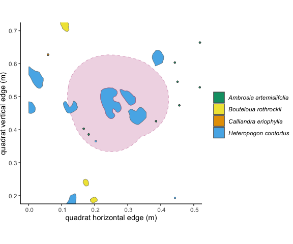
Figure 3.1: This individual outlined in pink is a focal individual, and the pale pink shows a 10 cm buffer around it.

Figure 3.2: The 10cm buffer around the focal individual overlaps with 5
other unique individuals of two species. These overlapping individuals
are outlined in dark grey. Using the ‘count’ method in
getNeighbors(), we would get an intraspecific competition
value of 3, and an interspecific competition value of 5.
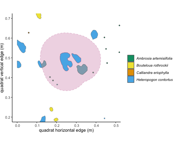
Figure 3.3: The 10cm buffer around the focal individual overlaps with 5
other unique individuals of two species. The overlapping area is shaded
in grey. Using the ‘area’ method in getNeighbors(), we
would get an intraspecific competition metric of 0.0454, and an
interspecific competition metric of 0.0462.
Below are the arguments in the getNeighbors()
function.
dat An sf data frame in
which each row represents data for a unique individual organism in a
unique year. The sf geometry for each row must be either
MULTIPOLYGON or POLYGON geometry. In addition
to a “geometry” column, this data frame must have columns that contain
data indicating the site, quadrat, site, and year of each observation.
There also must be a column that contains a unique identifying value for
each genet in each year. If dat is coming directly from
trackSpp(), this column will be called “trackID”.buff This is a single numeric value
that indicates the desired width of the “buffer” around the focal
individual in which the competitors are to be counted. This value must
be in the same units as the spatial information in
dat.method This is a character string that
must equal either "count" or "area". If
method = "count", then the number of individuals in the
buffer area will be tallied. If method = "area", then the
proportion of the buffer area that is occupied by other individuals will
be calculated.compType This is a character string
that must be either "allSpp" or "oneSpp". If
compType = "allSpp", then a metric of interspecific
competition is calculated, meaning that every individual within the
buffer around the focal individual is considered, no matter the species.
If compType = "oneSpp", then a metric of intraspecific
competition is calculated, meaning that only individuals of the same
species as the focal individual will be considered when calculating the
competition metric. If no value is provided, it will default to
“allSpp”.output This is a character string that
is set to either "summed" or "bySpecies". The
default is "summed". This argument is only important to
consider if you are using compType = "allSpp". If
output = "summed", then only one count/area value is
returned for each individual. This value is the total count or area of
all neighbors within the focal species buffer zone, regardless of
species. If output = "bySpecies", there is a count or area
value returned for each species present in the buffer zone. For example,
you are using getNeighbors() with
method = "count" and compType = "allSpp". A
focal individual in your dataset has seven other plants inside its
buffer zone, three of species A, two of species B, and 2 of species C.
If output = "summed", the value in the “neighbors_count”
column of the returned data frame will simply contain the value “7”. If
output = "bySpecies", the “neighbors_count” column for this
individual will actually contain a named list
{r} list("Species A "= 5, "Species B" = 3, "Species C" = 7).
The default value of output is "summed".trackID/species/quad/year/site/geometry
These arguments only need to be included if the columns in
dat that contain the data for trackID, species, site,
quadrat, year and geometry of each observation are different
from the names “trackID,”Species”, “Site”, “Quad”, “Year, and”geometry”.
For example, if the column in your version of dat that
contains the species identity of each observation is called
“species_names”, then the argument
species = "species_names" must be included in your call to
getNeighbors().The output of getNeighbors() is an sf data
frame that is identical to the input dat, but with either
one or two additional columns. If method = "area", there
are two columns added called “nBuff_area” and “neighbors_area”. The
first contains the area of the buffer zone around each focal individual.
The second contains the basal area of neighbors that overlap with a
focal individual’s buffer zone. If method = "count", there
is only one additional column added to the output, called
“neighbors_count.” This column contains a count of the neighbors that
occur within a focal individual’s buffer zone.
Here’s an example of a getNeighbors() function call
using the resulting data from the example in section 2.2, as
well as the resulting data frame. Note that
method = "area", so two columns are added to the returned
data frame:
datNeighbors <- plantTracker::getNeighbors(dat = datTrackSpp,
             buff = .15,
             method = "area",
             compType = "allSpp")
#> Simple feature collection with 477 features and 14 fields
#> Geometry type: GEOMETRY
#> Dimension: XY
#> Bounding box: xmin: -0.001386579 ymin: -0.001017592 xmax: 1.000536 ymax: 1.001267
#> CRS: NA
#> First 10 features:
#> Species Site Quad trackID Year neighbors_area
#> 1 Ambrosia artemisiifolia AZ SG2 AMBART_1922_1 1922 0.0011328591
#> 2 Ambrosia artemisiifolia AZ SG2 AMBART_1922_10 1922 0.0040518140
#> 3 Ambrosia artemisiifolia AZ SG2 AMBART_1922_11 1922 0.0055774468
#> 4 Ambrosia artemisiifolia AZ SG2 AMBART_1922_12 1922 0.0029129080
#> 5 Ambrosia artemisiifolia AZ SG2 AMBART_1922_13 1922 0.0050297901
#> 6 Ambrosia artemisiifolia AZ SG2 AMBART_1922_14 1922 0.0037646754
#> 7 Ambrosia artemisiifolia AZ SG2 AMBART_1922_15 1922 0.0026270846
#> 8 Ambrosia artemisiifolia AZ SG2 AMBART_1922_16 1922 0.0013297048
#> 9 Ambrosia artemisiifolia AZ SG2 AMBART_1922_17 1922 0.0022690175
#> 10 Ambrosia artemisiifolia AZ SG2 AMBART_1922_18 1922 0.0006338116
#> nBuff_area basalArea basalArea_genet survives_t+1 survives_tplus1 size_t+1
#> 1 0.04344697 point 2.461883e-05 NA 0 NA
#> 2 0.07329218 point 2.461883e-05 NA 0 NA
#> 3 0.07329218 point 2.461883e-05 NA 0 NA
#> 4 0.07329218 point 2.461883e-05 NA 0 NA
#> 5 0.07329218 point 2.461883e-05 NA 0 NA
#> 6 0.07329218 point 2.461883e-05 NA 0 NA
#> 7 0.07329218 point 2.461883e-05 NA 0 NA
#> 8 0.07329218 point 2.461883e-05 NA 0 NA
#> 9 0.06848976 point 2.461883e-05 NA 0 NA
#> 10 0.07329218 point 2.461883e-05 NA 0 NA
#> size_tplus1 nearEdge geometry
#> 1 NA TRUE POLYGON ((0.350604 0.021361...
#> 2 NA FALSE POLYGON ((0.7172048 0.25834...
#> 3 NA FALSE POLYGON ((0.1845598 0.38566...
#> 4 NA FALSE POLYGON ((0.759387 0.399850...
#> 5 NA FALSE POLYGON ((0.1696044 0.40291...
#> 6 NA FALSE POLYGON ((0.7290925 0.41097...
#> 7 NA FALSE POLYGON ((0.6255546 0.45737...
#> 8 NA FALSE POLYGON ((0.5872073 0.46925...
#> 9 NA FALSE POLYGON ((0.8863168 0.52256...
#> 10 NA FALSE POLYGON ((0.5212498 0.52831...The example above uses the option output = "summed",
which is the default for the getNeighbors() function. With
this option, the “neighbors_area” or “neighbors_count” column (depending
on the method argument) contains just one value that sums
the neighbor count or area across all neighbor species. However, if
output = "bySpecies", the “neighbors_count” or
“neighbors_area” column contains a list with the counts or areas broken
down by species. The output argument is described in more
detail in section 3.1. If you want to use the
getNeighbors() function to determine how the effect of
neighbors differs according to the species identity of those neighbors,
setting output = "bySpecies" allows you to do this.
However, it is likely that your subsequent analyses will need the
by-species neighbor data in a matrix or data frame format, rather than
in a list nested inside a data frame, which is how
getNeighbors() returns the data.
Here is some code that turns the data returned by
getNeighbors(output = "bySpecies") into a matrix where each
row has data for one focal individual, and each column has data for one
species. This format should be easier to work with for further
analysis.
# save the output of the getNeighbors() function
datNeighbors_bySpp <- plantTracker::getNeighbors(dat = datTrackSpp,
             buff = .15, method = "area", compType = "allSpp", output = "bySpecies")

# determine all of the possible species that can occupy the buffer zone
compSpp <- unique(datTrackSpp$Species)

temp <- lapply(X = datNeighbors_bySpp$neighbors_area,  FUN = function(x) {
  tmp <- unlist(x)
  tmp2 <- tmp[compSpp]
  }
)

for (i in 1:length(temp)) {
  # fix the column names
  names(temp[[i]]) <- compSpp
  # save the data in a matrix
  if (i == 1) {
    datOut <- temp[[i]]
  } else {
    datOut <- rbind(datOut, temp[[i]])
  }
}
# make the rownames of the matrix correspond to the trackID of the focal individual
rownames(datOut) <- datNeighbors_bySpp$trackID

# show the first few rows of the datOut data frame:
datOut[1:5,]
#>                Ambrosia artemisiifolia Bouteloua rothrockii
#> AMBART_1922_1             4.923767e-05         5.216672e-04
#> AMBART_1922_10            8.437672e-05         1.250163e-03
#> AMBART_1922_11            2.461883e-05         2.310445e-04
#> AMBART_1922_12            9.353468e-05         7.408342e-04
#> AMBART_1922_13            2.461883e-05         1.906272e-08
#>                Calliandra eriophylla Heteropogon contortus
#> AMBART_1922_1                     NA          0.0005619542
#> AMBART_1922_10                    NA          0.0027172740
#> AMBART_1922_11                    NA          0.0053217835
#> AMBART_1922_12                    NA          0.0020785392
#> AMBART_1922_13 NA 0.0050051522At this point, this dataset should be ready for you to use in any applications wish! There are a few additional functions that may help you in your analyses, and these are outlined in this section.
getRecruits() functiongetLambda() functiongetBasalAreas() functiondrawQuadMap()
functionSpecific instructions for how to use each of these functions can be found in their documentation!