

This README is closely related to a publication in Methods in Ecology and Evolution (Husmann et al. 2022). When managing ecosystems, the question arises as to how to simultaneously combat biodiversity loss and maintain ecosystem functioning while improving human welfare. Designing multifunctional landscapes means deciding upon the composition and configuration of land-cover types, given that landscape patterns drive the landscape`s ecological value and its ability to satisfy societal demands. Land-cover allocation models, particularly optimization approaches, have proven helpful in revealing trade-offs between multiple objectives and services provided by different land-cover compositions.
The R package optimLanduse provides functions for easy and systematic applications of the robust multiobjective land-cover composition optimization approach of Knoke et al. (2016). It includes tools to determine the land-cover composition that best balances the multiple functions and services a landscape can provide, as well as tools for a deeper understanding and visualization of the contributions of the distinct indicators. The method has been developed and applied previously in a couple of studies, with some examples to be found in the Literature section. The methodological background of the approach can, e.g., be found in Knoke et al. (2016) and Husmann et al. (2022). We here refer to the nomenclature of Husmann et al. (2022). The package opens the approach of Knoke et al. (2016) to the community of landscape planners and provides opportunities for systematic or batch applications. To further enhance this, we have designed a shiny dashboard for the package to get a brief idea of its functionalities and to facilitate the usage of the package, see http://rshiny.gwdg.de/apps/optimLanduse/. The current package version optimizes land-cover compositions, but aspects of configuration may be added in the future.
This chapter provides a brief overview of the package functions (Fig. 1). For detailed information on methodological background, functions, and workflow please also refer to Husmann et al. (2022). We further refer the reader to the respective help pages of the package for more information.
The stable version of the package can be installed using the CRAN server. The development version can be found on the GitHub project page.
# If not already installed
#install.packages("optimLanduse")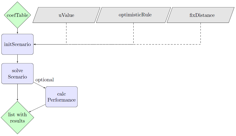
Fig. 1: Overview of the functions of the optimLanduse package. Green diamonds: input and output data; blue rectangles: functions; gray parallelograms: optional function settings.
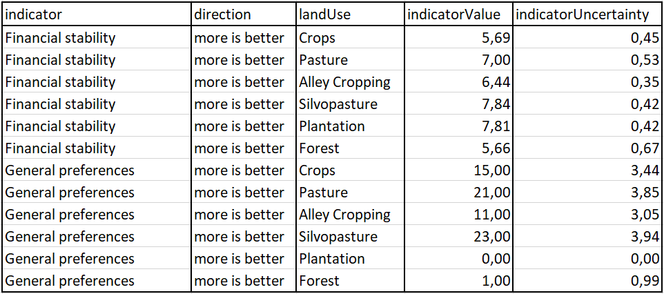
The initScenario() function combines the user settings with the data into an optimLanduse-object ready for solving. The following input data are required:
Table 1: Example of the data set from Gosling et al. (2020) to illustrate the required data structure.
uValue: The argument for the uncertainty level (\(f_u\), Equation 4 in Husmann et al., 2022). A higher uValue reflects a higher risk aversion of the decision maker. See the help file of the initScenario() function for more details.
optimisticRule: Specifies whether the optimistic contributions of each indicator should be defined either directly by their average, or by their average plus their uncertainty (if more is better) or minus their uncertainty (if less is better). The former option is most frequently used in recent literature and therefore builds the default.
fixDistance: Optional numeric value that defines distinct uncertainty levels for the calculation of the uncertainty space and the averaged distances of a certain land-cover composition (see Equation 9 in Husmann et al., n. d.). Passing NA disables fixDistance. The uncertainty space is then defined by the uValue.
The solveScenario() function takes the initialized optimLanduse-object and only a few optional solver-specific arguments.
digitsPrecision: Provides the only possibility for the user to influence the calculation time. As the solving process has no stochastic element, the calculation times depend almost only on the number of digits calculated only.
lowerBound & upperBound: Optional bounds for the land-cover alternatives. The lower bound must be 0 or a vector with lower bounds in the dimension of the number of land-cover alternatives. The upper bound, respectively, must be 1 or a vector with upper bounds. Choosing 0 and 1 (the defaults) as boundaries for all decision variables, means that no land-cover alternative is forced into the portfolio and that no land-cover alternative is assigned a maximum.
The returned list with results contains different information on the optimization model. It first repeats the settings of the initScenario(). These include:
This is followed by a summary of the results of the optimization:
The calcPerformance() function attaches the portfolio performances of all indicators and scenarios as a data frame to the solved optimLanduse object. The data can be used for straightforward visualization of the performance (e.g. Fig. 3). The performance is defined as the relative distance to the maximum achievable level for each indicator and uncertainty scenario. It calculates as 1 - \(d_{iu}\) (Equation 8, Husmann et al., 2022)
The autoSearch() function generates a list of all possible indicator combinations given in coefTable with their respective optimization results and the result that identifies the indicators that are best describing the currently observed land-use portfolio. The indicator combinations are exported as a list, where each combination corresponds to a list entry. For each of these list entries, an optimization is performed using the initScenario() and solveScenario() functions of the package. The result is saved into the respective list entry. In addition, each entry is appended with the currently observed land-use portfolio and the land-use portfolio when all indicators are optimized together. This list can than be filtered and ordered to e. g. identify different potential transformation pathway and trade-offs and synergies between them. To allow the user the same option settings, the initScenario() arguments uValue, optimisticRule and fixDistance can be adjusted. The landUseObs has to be a data frame with two columns. The first column has to contain the land-use options. The second column the respective shares.
Each of the returned list contains different information, these include:
We here present the basic workflow on a literature example. The aim of this chapter is to introduce the functionality of the packages’ functions and to explain the most relevant in- and outputs on the example of a use-case in Eastern Panama. The data of this study can be accessed in Appendix A of Gosling et al. (2020) and is also firmly integrated into the optimLanduse package. The exampleData(“exampleGosling.xlsx”) function helps loading the data in the environment. The data integrated in the package already comes in the required optimLanduse format, so that it can be used without any data processing.
Enriching agricultural farms with agroforestry has been promoted as a means to enhance ecosystem functioning in farms in Panama, while maintaining important economic functions. Gosling et al. (2020) therefore used the here presented optimization model to understand smallholder farmer’s perceptions and values of agroforestry systems. They identified 10 relevant indicators for a predefined set of land-cover alternatives, which represent the farmer’s goals (such as long and short-term income or labor demand, as well as carbon and water regulation). A survey with local farmers provided the empirical basis in the form of the farmer’s expectations on the indicator performance of each land-cover (arithmetic mean) and its uncertainties (using the standard error of the mean across the survey’s respondents). Descriptions of the land-cover alternatives and indicators can be found in Tables 1 and 2 in Gosling et al. (2020).
Loading Required Packages and Importing the Data
library(optimLanduse)
library(readxl)
library(future.apply) ## required only for autoSearch()-function
library(ggplot2)
library(tidyverse)
library(ggsci)

# Loading the example data
path <- exampleData("exampleGosling.xlsx")
dat <- read_excel(path)
dat is in the required format. Refer to the help of the initScenario() function or to the Initialization and Input chapter for more details.
Initializing an optimLanduse Object
# Initializing an optimLanduse-object
init <- initScenario(coefTable = dat,
                     uValue = 2,
                     optimisticRule = "expectation",
                     # optimistic contribution of each indicator directly defined
                     # by their average
                     fixDistance = NA)
                     # 3 is the default
In line with Gosling et al. (2020), we chose the expected value of the indicators as optimistic outcomes (optimisticRule = “expectation”) and the same uncertainty level for the calculation of the averaged distances and the uncertainty space (fixDistance = NA, see Equations 4 and 9 in Husmann et al., 2022 for more details).
Solving the Initialized optimLanduse Object
# Solve the initialized optimLanduse object using the solveScenario() function
result <- solveScenario(x = init)

# Visualize the farm composition
result$landUse %>% gather(key = landCoverOption,
                          value = landCoverShare) %>%
  ggplot(aes(y = landCoverShare*100, x="", fill = landCoverOption)) +
   geom_bar(position = "stack", stat = "identity") +
   theme_classic() +
   scale_fill_startrek() +
   xlab("Optimal land-use composition")+
   ylab( "Allocated share (%)") +
   theme(text = element_text(size = 14),
         legend.title=element_blank()) +
  scale_y_continuous(breaks = seq(0, 100, 10),
                     limits = c(0, 100))
Fig. 2: Composition of the optimized farm (based on data of Gosling et al. (2020)), including all indicators. Each land-cover option is shown in an allocated share (%).
The resulting optimized farm composition (Fig. 2) corresponds to Fig. 3 (\(f_u=2\)) in Gosling et al. (2020). It can be seen that the farm composition that best contributes to all 10 indicators (i.e. the multifunctional portfolio) is dominated by silvopasture and forest. According to Gosling et al. (2020), this reveals the potential of agroforestry to serve as a compromised solution to fulfill multiple ecological and economic functions. Recently, however, the observed average farm portfolio of the surveyed farms was mainly composed of pasture and cropland with only a small share of forest (14%). This reveals that not all of the selected objectives currently drive farmer’s land-cover decisions. The optimization approach can then be used to dive deeper into the effect of different goals on the resulting optimized land-cover composition and the effects of uncertainty.
Calculating the Portfolio Performances of the Optimized optimLanduse Object
# Performance calculations
performance <- calcPerformance(result)

performance$scenarioTable$performance <- performance$scenarioTable$performance * 100

ggplot(performance$scenarioTable,
       aes(x = indicator,
           y = performance,
           color = indicator)) +
  geom_point() +
  geom_hline(yintercept =
               min(performance$scenarioTable$performance),
             linetype = "dashed", color = "red") +
  guides(color = guide_legend(title = "",
                              nrow = 10)) +
  theme_classic() +
  theme(text = element_text(size = 18),
        legend.position="right",
        axis.ticks.x = element_blank()) +
  scale_x_discrete(labels = seq(1, 10)) +
  labs(y = "Min-max normalized indicator value (%)",
       x = "Indicators") +
  scale_y_continuous(breaks = seq(0, 101, 10),
                     limits = c(0, 101)) +
  geom_hline(aes(yintercept=100), size = 1) +
  annotate(geom = "Text", x = 6, y = 100, label = "Maximum achievable indicator level",
           vjust = -1)
Fig. 3: The performances of each of the 10 indicators for the ideal farm composition. The colored points are the achieved levels of the indicators of all scenarios. The dotted, horizontal red line illustrates the guaranteed performances \((1-\beta)\), and thus the robust feasible solution of the program (Equation 1 in Husmann et al, 2022).
Fig. 3 can be used to further explore the effects of the indicators on the modeled land-cover decisions. Looking at the performances of this multifunctional farm reveals which indicator equals \(\beta\) and therefore defines the result (Equation 1 in Husmann et al., 2022).
Here, the worst performing scenarios of indicators 1 (financial stability), 3 (investment costs) and 8 (meeting household needs) have equally the largest distances. It can be seen that the portfolio appears to be driven by these 3 indicators. In the worst-performing uncertainty scenarios, these 3 indicators show the maximum distances across all indicators. In other words, the guaranteed performance \(1-\beta\) of the portfolio is defined by these 3 indicators. A full list with performances of all individual scenarios is provided by the output scenarioTable after using the calcPerformance() function (Table 2).
It follows that these 3 indicators are crucial when discussing future land-cover alternatives and concepts. According to Gosling et al. (2020), this result is in line with current observed behavior since the need for short-term liquidity mainly drives smallholder farmers’ decisions in the study region. Intermediate-term economic success is not relevant until household consumption is secured. While the performances of indicator 1 differ relatively strongly among the scenarios, the performances of indicators 3 and 8 are quite similar within all scenarios. This is attributed to the larger standard errors of this indicator. Thus, it may be worth investigating the particular reasons behind this high uncertainty for indicator 1.
performance$beta## [1] 0.6132performanceExample <- head(performance$scenarioTable[,c(1 : 8, 31)], n = 4)
knitr::kable(performanceExample, row.names = F)Table 2: An extract of the scenario table of all indicators created through the calcPerformance() function with the worst performing scenarios
| indicator | outcomeCrops | outcomePasture | outcomeAlley Cropping | outcomeSilvopasture | outcomePlantation | outcomeForest | direction | performance |
|---|---|---|---|---|---|---|---|---|
| Financial stability | High | High | High | High | High | High | more is better | 61.31992 |
| Financial stability | Low | High | High | High | High | High | more is better | 72.31477 |
| Financial stability | High | Low | High | High | High | High | more is better | 61.31992 |
| Financial stability | Low | Low | High | High | High | High | more is better | 72.31477 |
Comparison of the Performance of the Currently Observed Land-cover Composition to the Optimized Composition
result_current <- solveScenario(x = init,
                                lowerBound = c(0.26, 0.59, 0, 0, 0.01, 0.14),
                                upperBound = c(0.26, 0.59, 0, 0, 0.01, 0.14))

performance_current <- calcPerformance(result_current)

performance_current$scenarioTable$performance <-
performance_current$scenarioTable$performance * 100performance_current$beta## [1] 0.9114ggplot(performance_current$scenarioTable,
aes(x = indicator,
y = performance,
color = indicator)) +
geom_point() +
geom_hline(yintercept =
min(performance_current$scenarioTable$performance),
linetype = "dashed", color = "red") +
guides(color = guide_legend(title = "",
nrow = 10)) +
theme_classic() +
theme(text = element_text(size = 18),
legend.position="right",
axis.ticks.x = element_blank()) +
scale_x_discrete(labels = seq(1, 10)) +
labs(y = "Min-max normalized indicator value (%)",
x = "Indicators") +
scale_y_continuous(breaks = seq(0, 101, 10),
limits = c(0, 101)) +
geom_hline(aes(yintercept=100), size = 1) +
annotate(geom = "Text", x = 6, y = 100, label = "Maximum achievable indicator level",
vjust = -1)
Fig. 4: The performance of each of the 10 indicators for the result of the currently observed land-cover composition. The colored points are the achieved levels of the indicators of all scenarios s. The dotted, horizontal red line illustrates the guaranteed performance \((1-\beta)\), thus the robust feasible solution of the program (Equation 1 in Husmann et al., 2022).
Setting the arguments for the lower and upper bounds exactly to the currently observed land-cover composition forces a solution that corresponds to the current land-cover composition (Fig. 4). It allows for the comparison and evaluation of the differences of the optimized land-cover composition with the currently observed composition. Comparing, e.g., the guaranteed performances \(1-\beta\) provides an objective measure of how an optimization enhances the achievements of the overall performance. A deeper look at the performances of the indicators reveals which indicators particularly benefit from optimization. Due to the compromise nature of the approach, indicators can also perform worse in the optimized portfolio when compared to the current land-cover composition.
Amounting to 0.387, the guaranteed performance of the multifunctional portfolio is considerably higher than the guaranteed performance of the current land-cover composition (0.089). In the optimized portfolio, each of the indicators considered is thus fulfilled by at least 38.7% compared to its individual achievable level. The comparison of the performances of the currently observed land-cover composition (Fig. 4) with the performances of the multifunctional portfolio (Fig. 3) reveals that, for example, the performance of the financial stability is significantly higher in the optimized portfolio. The performance of meeting households needs and liquidity, for example, decreases significantly. The price to be paid for the best-possible compromise is thus a fundamentally lower performance of both indicators that approximate the immediate economic success. The generally desirable multifunctional portfolio therefore does not promise immediate economic success for the farmers.
Calculating a List of all possible Indicator Combinations and their Respective Optimization Result
# Select evaluation strategy
plan(multisession)

# Define data frame for observed land-use shares
obsLU <- data.frame(landUse = c("Pasture", "Crops", "Forest", "Plantation",
                                "Alley Cropping", "Silvopasture"),
                    share = c(0.59, 0.26, 0.14, 0.01, 0, 0))
Table 3: Example of the structure needed for the obsLU argument
| landUse | share |
|---|---|
| Pasture | 0.59 |
| Crops | 0.26 |
| Forest | 0.14 |
| Plantation | 0.01 |
| Alley Cropping | 0.00 |
| Silvopasture | 0.00 |
First, we choose the evaluation strategy. In this example, we decided to run the calculations in parallel on the local machine plan(multisession). This greatly reduces the calculation time. It also allows developers to modify the function for larger data sets that quickly become time-intensive and run it on, for example, high-performance computing (HPC). In addition, a data frame must be created that shows the different land-cover types in the first column and the respective observed land-cover shares in the second column (see Table 3).
combList <- autoSearch(coefTable = dat,
                       landUseObs = obsLU,
                       uValue = 2,
                       optimisticRule = "expectation",
                       fixDistance = NA)
# End the parallelization process
plan(sequential)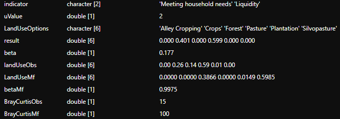
Figure 5: Example of the resulting list from the autoSearch() function to illustrate the elements.
The list combList contains two sub-lists. The first contains the result that best describes the currently observed land-cover decision. The second contains all indicator combinations (Fig. 5). In our example, 2^10 -1 combinations (Equation ??? in von Groß et al., 2023). To compare the land-cover types of the different indicator combinations with those of the currently observed and with the portfolio that optimizes all indicators simultaneously, the Bray-Curtis measure of dissimilarity is used (for more details, see Equation ??? in von Groß et al., 2023). This detailed list of all indicator combinations, their respective optimization results and their comparison to the the currently observed portfolio and the portfolio that optimizes all indicators simultaneously can be used for e. g. identifying different potential transformation pathway and trade-offs and synergies between them (Section ??? in von Groß et al., 2023).
applyDf <- data.frame(u = seq(0, 3, .5))

applyFun <- function(x) {
  init <- initScenario(dat, uValue = x, optimisticRule = "expectation", fixDistance = NA)
  result <- solveScenario(x = init)
  output <- c(result$beta, as.matrix(result$landUse))
  names(output) <- c("beta", names(result$landUse))
  return(output)
}

applyDf <- cbind(applyDf,
                 t(apply(applyDf, 1, applyFun)))

applyDf[, c(3 : 8)] <- applyDf[, c(3 : 8)] * 100

applyDf %>% gather(key = "land-cover option", value = "land-cover share", -u, -beta) %>%
  ggplot(aes(y = `land-cover share`, x = u, fill = `land-cover option`)) +
  geom_area(alpha = .8, color = "white") + theme_minimal()+
  labs(x = "Uncertainty level", y = "Allocated share (%)") +
  guides(fill=guide_legend(title="")) +
  scale_y_continuous(breaks = seq(0, 100, 10),
                     limits = c(0, 100.01)) +
  scale_x_continuous(breaks = seq(0, 3, 0.5),
                     limits = c(0, 3)) +
  scale_fill_startrek() +
  theme(text = element_text(size = 18),
        legend.position = "bottom")
Fig. 6: Theoretically ideal farm compositions under increasing levels of uncertainty.
Solving the portfolio (Fig. 6) under increasing assumptions for the uncertainty levels (uValue, respectively \(f_u\) in Equation 4 in Husmann et al., 2022) provides the sensitivity of the land-cover compositions to an increasing risk aversion of the farmers. Fig. 6 corresponds to Fig. 3 in Gosling et al. (2020). The higher the uncertainty level, the higher the uncertainty spaces of the indicators. Here, the composition of land-cover alternatives is relatively stable across different uncertainty levels (Fig. 6). An uValue of 0 leads to Portfolios without consideration of risk. Here, the results corresponds to an ordinary (non-robust) reference point approach. Comparing portfolios of uValue 0 with uValue 3, the share of forest decreases slightly from 41.2% to 34.3% and silvopasture from 45.9% to 44.9%. The share of crops decreases from 12.9% to 1%. At the same time, the shares of pasture increased from 0% to 9.6% and that of plantation from 0% to 10.2%.
Alley cropping does not appear in any portfolio at any uncertainty level. It does not, on average, contribute best to any indicator (Table 1 in Husmann et al., 2022). At least one other land-cover type contributes better to each indicator. It also contributes the worst (highest) to management complexity. This overall negative contribution does not change with increasing uncertainty levels. By trend, higher uncertainty levels lead to more diverse portfolios. The uncertainty spaces of all indicators increase with increasing uncertainty levels. These broadened individual uncertainty spaces then lead to a broader state space with a higher number of possible candidates for lowest-performing scenarios (i.e., scenarios that can under lower uncertainty not become part of the solution, as their distances could not be the maximum distance of any land-cover composition). Plantation, for example, is not part of the portfolio till an uncertainty level of 1.5. Plantation only provides the best to the long-term income while providing by far the worst to the general preferences. It also only provides minor contributions to the indicators. Under an uncertainty level of 1, for example, plantation provides the worst to the general preferences even if all other indicators are considered as worst-possible contributions. This ranking changes after uncertainty levels of 1.5 and above. At uncertainty level of 1.5, the worst-possible contribution of forests to the general preferences (\(1 - 0.99 * 2 = -0.98\), see Table 1 in Husmann et al., 2022) is then the worst possible contributing indicator among all land-cover types.
The sensitivity of the land-cover compositions towards indicators or groups of indicators can be analyzed by either excluding or adding indicators and interpreting the differences in the results of the distinct optimizations. To do so, individual and independent optimizations are carried out in- and excluding different (sets of) indicators. The set of indicators considered is representative of the stakeholders’ preferences and perceptions. Comparison of optimal land-cover compositions under differing indicator combinations may help to understand how stakeholders’ preferences design the land-cover compositions. The following code exemplifies optimizations for three subsets of indicators presented in Gosling et al. (2020). The shiny app of optimLanduse (http://rshiny.gwdg.de/apps/optimLanduse/) provides straightforward functionality to define sets of indicators with a single click. Further explanation and instructions are given in the app.
dat_socioeconomic <- dat[!dat$indicator %in% c("Protecting soil resources",
                                               "Protecting water supply"),]

init_socioeconomic <- initScenario(dat_socioeconomic,
                                   uValue = 2,
                                   optimisticRule = "expectation",
                                   fixDistance = NA)

result_socioeconomic <- solveScenario(x = init_socioeconomic)

result_socioeconomic$landUse %>% gather(key = landCoverOption,
                                        value = landCoverShare, 1 : 6) %>%
  mutate(portfolio = "Socio-economic",
         landCoverShare = landCoverShare * 100) %>%
  ggplot(aes(y = landCoverShare, x = portfolio, fill = landCoverOption)) +
  geom_bar(position = "stack", stat = "identity") +
  theme_classic() +
  theme(text = element_text(size = 14)) +
  scale_fill_startrek() +
  labs(y = "Allocated share (%)") +
  scale_y_continuous(breaks = seq(0, 100, 10),
                     limits = c(0, 100)) +
  theme(axis.title.x=element_blank(),
        axis.ticks.x=element_blank()) +
  guides(fill=guide_legend(title=""))
Fig. 7: Composition of the optimized farm (based on data of Gosling et al., 2020), including only socio-economic indicators. Each land-cover option is shown in an allocated share (%).
The first example considers socio-economic indicators only (Fig. 7; see also Fig. 5 of Gosling et al., 2020). The result corresponds to the above shown multifunctional portfolio (Fig. 2). This is expected, as all indicators relevant to the solution of the multifunctional portfolio (financial stability, investment costs, and meeting household needs) are also captured in the socio-economic bundle.
performance_socioeconomic <- calcPerformance(result_socioeconomic)

performance_socioeconomic$scenarioTable$performance <-
  performance_socioeconomic$scenarioTable$performance * 100

performance_socioeconomic$beta
## [1] 0.6132ggplot(performance_socioeconomic$scenarioTable,
aes(x = indicator,
y = performance,
color = indicator)) +
geom_point() +
geom_hline(yintercept =
min(performance$scenarioTable$performance),
linetype = "dashed", color = "red") +
guides(color = guide_legend(title = "",
nrow = 10)) +
theme_classic() +
theme(text = element_text(size = 18),
legend.position="right",
axis.ticks.x = element_blank()) +
scale_x_discrete(labels = seq(1, 10)) +
labs(y = "Min-max normalized indicator value (%)",
x = "Indicators") +
scale_y_continuous(breaks = seq(0, 101, 10),
limits = c(0, 101)) +
geom_hline(aes(yintercept=100), size = 1) +
annotate(geom = "Text", x = 6, y = 100, label = "Maximum achievable indicator level",
vjust = -1)
Fig. 8: The performance of each of the socio-economic indicators. The colored points are the achieved levels of the indicators of all scenarios. The dotted, horizontal red line illustrates the guaranteed performance \((1-\beta)\), and thus the robust feasible solution of the program (Equation 1 in Husmann et al, 2022).
An analysis of the performance of the socio-economic indicators shows that the performances of the three relevant indicators equal the multifunctional portfolio (Fig. 8). The result is still defined by financial stability, investment costs and meeting household needs. Consequently, the guaranteed performance \((1-\beta)\) also equals the multifunctional portfolio. Therefore, this socio-economic portfolio also does not perfectly reflect the currently observed land-cover composition. This means that further indicators appear to be relevant for the actual farmer’s decisions.
dat_ecologic <- dat[dat$indicator %in% c("Protecting soil resources",
                                         "Protecting water supply"),]

init_ecologic <- initScenario(dat_ecologic,
                              uValue = 2,
                              optimisticRule = "expectation",
                              fixDistance = NA)

result_ecologic <- solveScenario(x = init_ecologic)

result_ecologic$landUse %>% gather(key = landCoverOption, value = landCoverShare, 1 : 6) %>%
  mutate(portfolio = "Ecologic",
         landCoverShare = landCoverShare * 100) %>%
  ggplot(aes(y = landCoverShare, x = portfolio, fill = landCoverOption)) +
  geom_bar(position = "stack", stat = "identity") +
  theme_classic() +
  theme(text = element_text(size = 14)) +
  scale_fill_startrek() +
  labs(y = "Allocated share (%)") +
  scale_y_continuous(breaks = seq(0, 100, 10),
                     limits = c(0, 100)) +
  theme(axis.title.x=element_blank(),
        axis.ticks.x=element_blank()) +
  guides(fill=guide_legend(title=""))
Fig. 9: Composition of the optimized farm (based on data of Gosling et al., 2020), including only ecological indicators. Each land-cover option is shown in an allocated share (%).
As the second example, the ecological indicator group leads to a land-cover portfolio comprising of only forests (Fig. 9; corresponds to Fig. 6 of Gosling et al., 2020). It can be concluded that all contributions of all other land-cover alternatives in all scenarios (even the optimistic ones) to the ecological indicators are lower than those of forests. The land-cover composition of the ecologic bundle differs fundamentally from the currently observed portfolio. The ecological indicators are therefore apparently not sufficient to approximate the farmer’s current perceptions.
dat_short <- dat[dat$indicator %in% c("Meeting household needs",
                                      "Liquidity"),]

init_short<- initScenario(dat_short,
                          uValue = 2,
                          optimisticRule = "expectation",
                          fixDistance = NA)

result_short <- solveScenario(x = init_short)

result_short$landUse %>% gather(key = landCoverOption, value = landCoverShare, 1 : 6) %>%
  mutate(portfolio = "Immediate",
         landCoverShare = landCoverShare * 100) %>%
  ggplot(aes(y = landCoverShare, x = portfolio, fill = landCoverOption)) +
  geom_bar(position = "stack", stat = "identity") +
  theme_classic() +
  theme(text = element_text(size = 14)) +
  scale_fill_startrek() +
  labs(y = "Allocated share (%)") +
  scale_y_continuous(breaks = seq(0, 100, 10),
                     limits = c(0, 100)) +
  theme(axis.title.x = element_blank(),
        axis.ticks.x = element_blank()) +
  guides(fill = guide_legend(title = ""))
Fig. 10: Composition of the optimized farm (based on data of Gosling et al., 2020), including the prospective relevant indicators of the farmers only. Each land-cover option is shown in an allocated share (%).
The third example is composed of a bundle of indicators that prospectively reflect the farmer’s needs and perceptions (Fig. 10). Corresponding to Fig. 6 of Gosling et al. (2020), this scenario only consists of indicators that approximate immediate economic success. Indeed, the land-cover composition of this portfolio best reflects the portfolio observed in Eastern Panama. Hence, these indicators presumably best reflect the farmer’s goals and perceptions in Eastern Panama. The difference between this portfolio and the desired multifunctional portfolio (Fig. 2) highlights the requirements a land-cover alternative must fulfill to meet the farmer’s requirements and goals. The silvopasture, as defined in Gosling et al. (2020), may not serve the requirements of the farmers sufficiently. Since farmers rate liquidity and meeting household needs higher than long-term profit and economic stability, pasture outperforms silvopasture in the immediate return scenario. Policies or development plans may consider these indicators as key elements when promoting landscape development toward multifunctional landscapes.
A pay-off matrix provides information about the influence of single indicators on the sensitivity of the results (see e.g. Aldea et al., 2014, Table 1; Ezquerro et al., 2019, Table 1; Knoke et al., 2020, Supporting Information Table S6). Originally, the pay-off matrix shows to which degree all indicators are fulfilled on average when the landscape is optimized for only one indicator. The average trade-offs between the one (optimized) indicator and all other (non-optimized) indicators are therewith shown. The fulfillment of these non-optimized indicators reveals synergies or antagonisms between the indicators. A robust pendant to this approach can be easily conducted with the optimLanduse package as the degrees of fulfillment are delivered straightaway using the calcPerformance() function.
In contrast to the original approach, each indicator has a set of performances (\(U_i\), Equations 2 and 3 in Husmann et al., 2022; Fig. 3 and 4 visualize the sets of indicator performances). Following the robust philosophy, we selected only the worst performance out of the set of uncertainties for each indicator. The resulting worst performances of the non-optimized indicators reveal the relative extent to which these indicators are fulfilled under the worst-case uncertainty scenario. It therewith reveals to which degree the indicators are antagonistic or synergistic. The indicator performances are expressed in relation to the best-possible fulfillment of the respective indicators (Equation 3 of Husmann et al., 2022). In contrast to the original approach, we thus calculate relative degrees of fulfillment for each indicator.
The following code calculates a pay-off matrix using the apply function. For this, payOffFun encloses all calculation steps. payOffFun expects the name of the indicator that is to be considered in the optimization x and the data in the optimLanduse format dat. In payOffFun, firstly (1), the land-cover composition is optimized considering only the indicator defined in x. The resulting land-cover composition is then (2) passed as lower and as upper bounds to the land-cover optimization that considers all indicators. Accordingly, the solution of the second optimization (2) is exactly the result of the first optimization taking into account the indicator x only. The second optimization only aims to prepare an optimLanduse object from which the performances of all indicators can be calculated. It delivers the performances of all indicators when only the indicator x is considered in the optimization. From each indicator’s set of calculated performances, only the minimum performance is selected (3) and then saved into the pay-off matrix. To sum up, each row of the pay-off matrix contains the minimum performances of all single indicators when the land-cover composition is optimized considering only one indicator. The name of this indicator considered in the optimization is written in the first column of each row. The names of all indicators are given in the table header. Consequently, the performances of the indicators considered are obligatorily best fulfilled so that the matrix’s main diagonal contains the highest value of each indicator.
# Initialize the optimization that considers all indicators outside of the
# apply function saves calculation time
init_payOff <- initScenario(coefTable = dat,
                            uValue = 2,
                            optimisticRule = "expectation",
                            fixDistance = NA)

# Initialize an empty pay-off matrix
payOffDf <- data.frame(indicator = unique(init_payOff$scenarioTable$indicator))

# Define the function for apply
payOffFun <- function(x, dat) {

  ## (1) Optimize the land-cover composition for the indicator x only ##

  # Filter for the indicator x
  indicator_filtered <- x
  dat_filtered <- dat[dat$indicator == indicator_filtered, ]

  # Conduct optimization considering the indicator x only

  init_filtered <- initScenario(coefTable = dat_filtered,
                                uValue = 2,
                                optimisticRule = "expectation",
                                fixDistance = NA)

  result_filtered <- solveScenario(x = init_filtered)

  ## (2) Optimize the land-cover composition for all indicators, limited ##
  ##     to the land-cover composition calculated in step (1)            ##

  result_payOff <- solveScenario(x = init_payOff,
                          lowerBound = result_filtered$landUse,
                          upperBound = result_filtered$landUse)

  performance_payOff <- calcPerformance(x = result_payOff)

  ## (3) Taking the minimum performances of each indicator ##

  performance_payOff_min <- performance_payOff$scenarioTable %>%
    group_by(indicator) %>%
    summarise(min = min(performance))

  return(round(performance_payOff_min$min, 3))
}

# Apply the calculation of the pay-off matrix
payOff_Matrix<- cbind(payOffDf,
                 t(apply(payOffDf, 1, payOffFun, dat = dat)))

names(payOff_Matrix) <- c("Indicators", payOff_Matrix$indicator)

knitr::kable(payOff_Matrix, row.names = F)
Table 4: Performances of all indicators when optimized for single indicators only (pay-off matrix). The indicators considered for optimization are located in the first row. The other entries in the rows contain the performances of the respective non-optimized indicators.
| Indicators | Financial stability | General preferences | Investment costs | Labour demand | Liquidity | Long-term income | Management complexity | Meeting household needs | Protecting soil resources | Protecting water supply |
|---|---|---|---|---|---|---|---|---|---|---|
| Financial stability | 0.805 | 0.371 | 0.007 | 0.122 | 0.492 | 0.881 | 0.072 | 0.346 | 0.231 | 0.466 |
| General preferences | 0.427 | 0.832 | 0.012 | 0.093 | 0.854 | 0.789 | 0.090 | 0.669 | 0.184 | 0.334 |
| Investment costs | 0.000 | 0.000 | 1.000 | 1.000 | 0.000 | 0.000 | 1.000 | 0.000 | 1.000 | 1.000 |
| Labour demand | 0.000 | 0.000 | 1.000 | 1.000 | 0.000 | 0.000 | 1.000 | 0.000 | 1.000 | 1.000 |
| Liquidity | 0.134 | 0.579 | 0.000 | 0.061 | 1.000 | 0.780 | 0.158 | 0.705 | 0.000 | 0.000 |
| Long-term income | 0.553 | 0.273 | 0.016 | 0.113 | 0.465 | 0.920 | 0.106 | 0.258 | 0.140 | 0.338 |
| Management complexity | 0.000 | 0.000 | 1.000 | 1.000 | 0.000 | 0.000 | 1.000 | 0.000 | 1.000 | 1.000 |
| Meeting household needs | 0.000 | 0.353 | 0.006 | 0.000 | 0.559 | 0.483 | 0.000 | 1.000 | 0.000 | 0.000 |
| Protecting soil resources | 0.000 | 0.000 | 1.000 | 1.000 | 0.000 | 0.000 | 1.000 | 0.000 | 1.000 | 1.000 |
| Protecting water supply | 0.000 | 0.000 | 1.000 | 1.000 | 0.000 | 0.000 | 1.000 | 0.000 | 1.000 | 1.000 |
It can be followed from the pay-off matrix (Table 4), that, e.g., liquidity and long-term income are fulfilled to high degrees when optimized considering the general preferences only (row 2). In contrast, farmer’s requirements regarding investment costs (0.012) and management complexity (0.09) are fulfilled poorly.
When optimized considering only the water supply protection (row 10), the indicators most relevant for the farmers (meeting household needs and Liquidity, Fig. 10) perform very poorly (0.0). This shows that the water supply function is clearly antagonistic to the farmer’s requirements.
It can be advantageous to define distinct uncertainty levels for the calculation of the distances to the maximum achievable level (the reference) \(d_{iu}\) (Equation 3 in Husmann et al., 2022) and the actual distances under a certain land-cover composition \(R_{liu}\) (Equation 5 in Husmann et al., 2022, see also Equation 9). Too narrow uncertainty spaces of \(R_{liu}\) could restrict the state space of the distances too strictly. The broader uncertainty spaces allow for higher freedom of \(R_{liu}\), which allows to cover more land-cover compositions. The distances are thus allowed to be higher. This usually results in a more similar composition of the land-cover composition with similar levels of uncertainty. The transitions between the portfolios under rising uncertainty values are smoother. The disadvantage of distinct uncertainty spaces is that the distances can no longer be straightforwardly interpreted. The distances calculated using different uncertainty spaces considered in the denominator and the counter of Equation 3 (Husmann et al., 2022) cannot be interpreted as a degree of fulfillment anymore.
#### uValue 3 ####
path <- exampleData("exampleGosling.xlsx")
dat <- read_excel(path)

applyDf <- data.frame(u = seq(0, 3, .5))

applyFun <- function(x) {
  init <- initScenario(dat, uValue = x, optimisticRule = "expectation", fixDistance = 3)
  result <- solveScenario(x = init)
  return(c(result$beta, as.matrix(result$landUse)))
}

applyDf <- cbind(applyDf,
                 t(apply(applyDf, 1, applyFun)))

names(applyDf) <- c("u", "beta", names(result$landUse))

applyDf[, c(3 : 8)] <- applyDf[, c(3 : 8)] * 100

applyDf %>% gather(key = "land-cover option", value = "land-cover share", -u, -beta) %>%
  ggplot(aes(y = `land-cover share`, x = u, fill = `land-cover option`)) +
  geom_area(alpha = .8, color = "white") + theme_minimal()+
  labs(x = "Uncertainty level", y = "Allocated share (%)") +
  guides(fill=guide_legend(title="")) +
  scale_y_continuous(breaks = seq(0, 100, 10),
                     limits = c(0, 100.01)) +
  scale_x_continuous(breaks = seq(0, 3, 0.5),
                     limits = c(0, 3)) +
  scale_fill_startrek() +
  theme(text = element_text(size = 18),
        legend.position = "bottom")
Fig. 11: Theoretically ideal farm compositions using the fixDistance argument and increasing levels of uncertainty.
It can be seen that the land-cover allocation transition under increasing uncertainty levels (Fig. 11) differs slightly from the multifunctional scenario shown above (Fig. 2). The here broadened state space leads to a higher share of pasture under low uncertainty levels as compared to the multifunctional portfolio above (Fig. 7).
Husmann, K., von Groß, V., Bödeker, K., Fuchs, J.M., Paul, C., Knoke, T. (2022): optimLanduse: A package for multiobjective land-cover composition optimization under uncertainty. Methods Ecol Evol. https://doi.org/10.1111/2041-210X.14000
Aldea, J., Martínez-Peña, F., Romero, C., Diaz-Balteiro, L. (2014): Participatory Goal Programming in Forest Management: An Application Integrating Several Ecosystem Services. Forests, 5, 3352-3371. https://doi.org/10.3390/f5123352
Ezquerro, M., Pardos, M., Diaz-Balteiro, L. (2019): Integrating variable retention systems into strategic forest management to deal with conservation biodiversity objectives. Forest Ecology and Management, 433, 585-593. https://doi.org/10.1016/j.foreco.2018.11.003
Gosling, E., Reith, E., Knoke T., Paul, C. (2020): A goal programming approach to evaluate agroforestry systems in Eastern Panama. Journal of Environmental Management, 261:110248. https://doi.org/10.1016/j.jenvman.2020.110248
Husmann, K., von Groß, V., Bödeker, K., Fuchs, J.M., Paul, C., Knoke, T. (2022): optimLanduse: A package for multiobjective land-cover composition optimization under uncertainty. Methods Ecol Evol., 00, 1 - 10 https://doi.org/10.1111/2041-210X.14000
Knoke, T., Paul, C., Hildebrandt, P. et al. (2016): Compositional diversity of rehabilitated tropical lands supports multiple ecosystem services and buffers uncertainties. Nat Commun 7, 11877. https://doi.org/10.1038/ncomms11877
Knoke, T., Paul, C., Rammig, A., et al. (2020): Accounting for multiple ecosystem services in a simulation of land-use decisions: Does it reduce tropical deforestation? Global Change Biology, 26(4), 2403-2420. https://doi.org/10.1111/gcb.15003
Paul, C., Weber, M., Knoke, T. (2017): Agroforestry versus farm mosaic systems – Comparing land-use efficiency, economic returns and risks under climate change effects. Sci. Total Environ., 587-588. https://doi.org/10.1016/j.scitotenv.2017.02.037