
![]()
The goal of logKDE is to provide a set of functions for kernel
density estimation on the positive domain, using log-kernel density
functions, for the R programming environment. The main
functions of the package are the logdensity and
logdensity_fft functions. The choice of functional syntax
was made to resemble those of the density function, for
conducting kernel density estimation on the real domain. The
logdensity function conducts density estimation, via first
principle computations, whereas logdensity_fft utilizes
fast-Fourier transformation in order to speed up computation. The use of
Rcpp guarantees that both methods are sufficiently fast for
large data scenarios.
Currently, a variety of kernel functions and plugin bandwidth methods
are available. By default both logdensity and
logdensity_fft are set to use log-normal kernel functions
(kernel = 'gaussian') and Silverman’s rule-of-thumb
bandwidth, applied to log-transformed data (bw = 'nrd0').
However, the following kernels are also available:
kernel = 'epanechnikov'),kernel = 'laplace'),kernel = 'logistic'),kernel = 'triangular'),kernel = 'uniform').The following plugin bandwidth methods are also available:
?bw.nrd regarding the
options),bw = 'logcv'),bw = 'logg').The logdensity and logdensity_fft functions
also behave in the same way as density, when called within
the plot function. The usual assortment of commands that
apply to plot output objects can also be called.
For a comprehensive review of the literature on positive-domain
kernel density estimation, thorough descriptions of the mathematics
relating to the methods that have been described, simulation results,
and example applications of the logKDE package, please
consult the package vignette. The vignette is available via the command
vignette('logKDE'), once the package is installed.
If devtools has already been installed, then the most
current build of logKDE can be obtained via the
command:
devtools::install_github('andrewthomasjones/logKDE',build_vignettes = T)The latest stable build of logKDE can be obtain from
CRAN via the command:
install.packages("logKDE", repos='http://cran.us.r-project.org')An archival build of logKDE is available at https://zenodo.org/record/1317784. Manual installation
instructions can be found within the R installation and
administration manual https://cran.r-project.org/doc/manuals/r-release/R-admin.html.
In this example, we demonstrate that logdensity has
nearly identical syntax to density. We also show that the
format of the outputs are also nearly identical.
## Load 'logKDE' library.
library(logKDE)

## Set a random seed.
set.seed(1)

## Generate strictly positive data.
## Data are generated from a chi-squared distribution with 12 degrees of freedom.
x <- rchisq(100,6)

## Construct and print the output of the function 'density'.
density(x)
#>
#> Call:
#>  density.default(x = x)
#>
#> Data: x (100 obs.);  Bandwidth 'bw' = 1.018
#>
#>        x                y
#>  Min.   :-2.366   Min.   :4.707e-05
#>  1st Qu.: 2.547   1st Qu.:7.209e-03
#>  Median : 7.459   Median :3.315e-02
#>  Mean   : 7.459   Mean   :5.079e-02
#>  3rd Qu.:12.372   3rd Qu.:1.012e-01
#>  Max.   :17.284   Max.   :1.311e-01

## Construct and print the output of the function 'logdensity'.
logdensity(x)
#>
#> Call:
#>  logdensity(x = x)
#>
#> Data: x (100 obs.);  Bandwidth 'bw' = 0.1923
#>
#>        x                 y
#>  Min.   : 0.1111   Min.   :0.00000
#>  1st Qu.: 3.7851   1st Qu.:0.02313
#>  Median : 7.4592   Median :0.06527
#>  Mean   : 7.4592   Mean   :0.06707
#>  3rd Qu.:11.1333   3rd Qu.:0.11219
#>  Max.   :14.8073   Max.   :0.13698

## Plot the 'density' output object.
plot(density(x))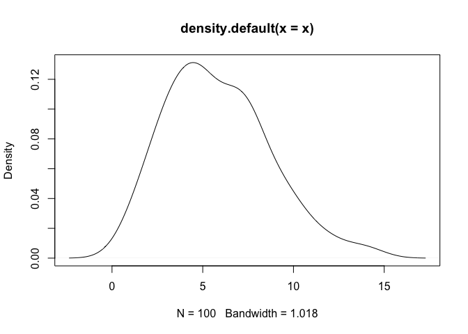
## Plot the 'logdensity' output object.
plot(logdensity(x))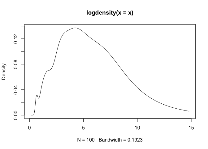
As a note, one can observe that density assigns positive
probability to negative values. Since we know that the chi-squared
generative model generates only positive values, this is an undesirable
result. The log-transformed kernel density estimator that is produced by
logdensity only assigns positive probability to positive
values, and is thus bona fide in this estimation scenario.
In this example, we showcase the variety of kernel functions that are
available in the package. Here, log-transformed kernel density
estimators are constructed using the logdensity
function.
## Load 'logKDE' library.
library(logKDE)

## Set a random seed.
set.seed(1)

## Generate strictly positive data.
## Data are generated from a chi-squared distribution with 12 degrees of freedom.
x <- rchisq(100,12)

## Construct a log-KDE using the data, and using each of the available kernel functions.
logKDE1 <- logdensity(x,kernel = 'gaussian',from = 1e-6,to = 30)
logKDE2 <- logdensity(x,kernel = 'epanechnikov',from = 1e-6,to = 30)
logKDE3 <- logdensity(x,kernel = 'laplace',from = 1e-6,to = 30)
logKDE4 <- logdensity(x,kernel = 'logistic',from = 1e-6,to = 30)
logKDE5 <- logdensity(x,kernel = 'triangular',from = 1e-6,to = 30)
logKDE6 <- logdensity(x,kernel = 'uniform',from = 1e-6,to = 30)

## Plot the true probability density function of the generative model.
plot(c(0,30),c(0,0.1),type='n',xlab='x',ylab='Density',main='Example 2')
curve(dchisq(x,12),from = 0,to = 30,add = T)

## Plot each of the log-KDE functions, each in a different rainbow() colour.
lines(logKDE1$x,logKDE1$y,col = rainbow(7)[1])
lines(logKDE2$x,logKDE2$y,col = rainbow(7)[2])
lines(logKDE3$x,logKDE3$y,col = rainbow(7)[3])
lines(logKDE4$x,logKDE4$y,col = rainbow(7)[4])
lines(logKDE5$x,logKDE5$y,col = rainbow(7)[5])
lines(logKDE6$x,logKDE6$y,col = rainbow(7)[6])

## Add a grid for a visual guide.
grid()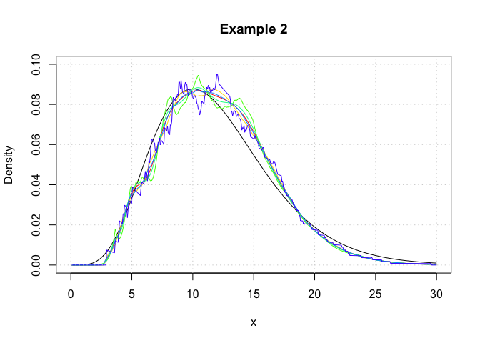
In this example, we show that logdensity and
logdensity_ftt yield nearly identical results. Here,
log-transformed kernel density estimators are constructed using the
logdensity_ftt function.
## Load 'logKDE' library.
library(logKDE)

## Set a random seed.
set.seed(1)

## Generate strictly positive data.
## Data are generated from a chi-squared distribution with 12 degrees of freedom.
x <- rchisq(100,12)

## Construct a log-KDE using the data, and using each of the available kernel functions.
logKDE1 <- logdensity_fft(x,kernel = 'gaussian',from = 1e-6,to = 30)
logKDE2 <- logdensity_fft(x,kernel = 'epanechnikov',from = 1e-6,to = 30)
logKDE3 <- logdensity_fft(x,kernel = 'laplace',from = 1e-6,to = 30)
logKDE4 <- logdensity_fft(x,kernel = 'logistic',from = 1e-6,to = 30)
logKDE5 <- logdensity_fft(x,kernel = 'triangular',from = 1e-6,to = 30)
logKDE6 <- logdensity_fft(x,kernel = 'uniform',from = 1e-6,to = 30)

## Plot the true probability density function of the generative model.
plot(c(0,30),c(0,0.1),type='n',xlab='x',ylab='Density',main='Example 3')
curve(dchisq(x,12),from = 0,to = 30,add = T)

## Plot each of the log-KDE functions, each in a different rainbow() colour.
lines(logKDE1$x,logKDE1$y,col = rainbow(7)[1])
lines(logKDE2$x,logKDE2$y,col = rainbow(7)[2])
lines(logKDE3$x,logKDE3$y,col = rainbow(7)[3])
lines(logKDE4$x,logKDE4$y,col = rainbow(7)[4])
lines(logKDE5$x,logKDE5$y,col = rainbow(7)[5])
lines(logKDE6$x,logKDE6$y,col = rainbow(7)[6])

## Add a grid for a visual guide.
grid()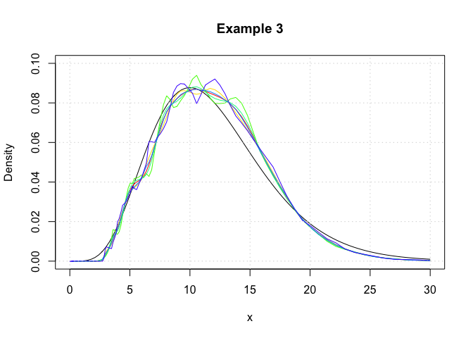
We observe that the logdensity_fft outputs are
noticiably smoother than those of logdensity. This is
because fast Fourier transformations (FFT) only yield kernel density
estimates at discrete points, and the regions between these discrete
points are approximated via a linear approximator, namely using the
approx function. This is the same evaluation technique as
that which is used in the function density. Additionally
the FFT approximation points are evenly space on the real line, whereas
those used for logdensity are evenly spaced on a log
scale.
In this example, we showcase the variety of plugin bandwidth
estimators that are available in the package. Here, log-transformed
kernel density estimators are constructed using the
logdensity function.
## Load 'logKDE' library.
library(logKDE)

## Set a random seed.
set.seed(1)

## Generate strictly positive data.
## Data are generated from a chi-squared distribution with 12 degrees of freedom.
x <- rchisq(100,12)

## Construct a log-KDE using the data, and using each of the available kernel functions.
logKDE1 <- logdensity(x,bw = 'nrd0',from = 1e-6,to = 30)
logKDE2 <- logdensity(x,bw = 'logcv',from = 1e-6,to = 30)
logKDE3 <- logdensity(x,bw = 'logg',from = 1e-6,to = 30)
logKDE4 <- logdensity(x,bw = 'nrd',from = 1e-6,to = 30)
logKDE5 <- logdensity(x,bw = 'ucv',from = 1e-6,to = 30)
#> Warning in stats::bw.ucv(log(x)): minimum occurred at one end of the range
logKDE6 <- logdensity(x,bw = 'bcv',from = 1e-6,to = 30)
#> Warning in stats::bw.bcv(log(x)): minimum occurred at one end of the range
logKDE7 <- logdensity(x,bw = 'SJ-ste',from = 1e-6,to = 30)
logKDE8 <- logdensity(x,bw = 'SJ-dpi',from = 1e-6,to = 30)


## Plot the true probability density function of the generative model.
plot(c(0,30),c(0,0.1),type='n',xlab='x',ylab='Density',main='Example 4')
curve(dchisq(x,12),from = 0,to = 30,add = T)

## Plot each of the log-KDE functions with different choices of bandwidth, each in a different rainbow() colour.
lines(logKDE1$x,logKDE1$y,col = rainbow(9)[1])
lines(logKDE2$x,logKDE2$y,col = rainbow(9)[2])
lines(logKDE3$x,logKDE3$y,col = rainbow(9)[3])
lines(logKDE4$x,logKDE4$y,col = rainbow(9)[4])
lines(logKDE5$x,logKDE5$y,col = rainbow(9)[5])
lines(logKDE6$x,logKDE6$y,col = rainbow(9)[6])
lines(logKDE7$x,logKDE7$y,col = rainbow(9)[7])
lines(logKDE8$x,logKDE8$y,col = rainbow(9)[8])

## Add a grid for a visual guide.
grid()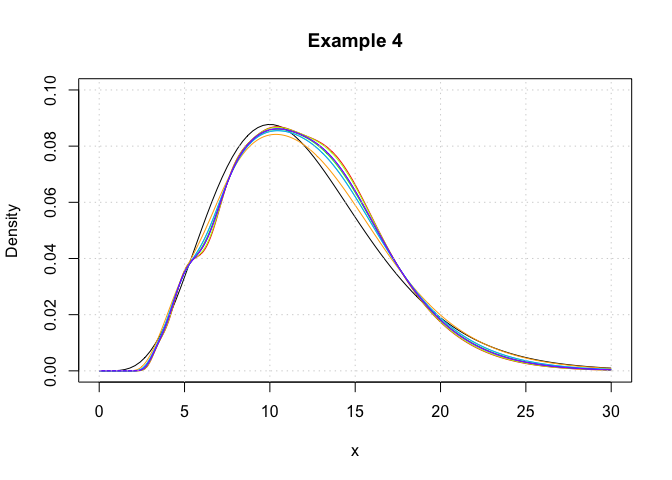
Using the package testthat, we have conducted the
following unit test for the GitHub build, on the date: 29 November,
2025. The testing files are contained in the tests
folder of the respository.
## Load 'logKDE' library.
library(logKDE)

## Load 'testthat' library.
library(testthat)
#> Warning: package 'testthat' was built under R version 4.4.1

## Test 'logKDE'.
test_package('logKDE')
#> [ FAIL 0 | WARN 0 | SKIP 0 | PASS 74 ]Thank you for your interest in logKDE. If you happen to
find any bugs in the program, then please report them on the Issues page
(https://github.com/andrewthomasjones/logKDE/issues).
Support can also be sought on this page. Furthermore, if you would like
to make a contribution to the software, then please forward a pull
request to the owner of the repository.