![]()
![]()
Calculations involving interest rates are usually very easy and
straightforward, but sometimes it involves specific issues that makes
the task of writing structured and reproducible code for it chalenging
and annoying. The fixedincome package brings many functions
to strucutre and create facilities to handle with interest rates, term
structure of interest rates and specific issues regarding compounding
rates and day count rules, for example.
Below there are a few examples on how to create and make calculations
with interest rates using fixedincome.
You can install from CRAN with:
install.packages("fixedincome")You can install the development version of fixedincome from GitHub with:
# install.packages("devtools")
devtools::install_github("wilsonfreitas/R-fixedincome")To create an interest rate we need to specify 4 elements:
simple, discrete or
continuous.actual/360 where the
days between two dates are calculated as the difference and the year is
assumed to be 360 days.actual calendar that compute the difference between
two dates.There is another important topic that wasn’t declared here that is
the frequency of interest. To start with the things simple
fixedincome handles only with annual rates since
this represents the great majority of rates used in financial market
contracts, but this restriction can be reviewed in the future.
Given that let’s declare an annual spot rate with a
simple compounding, an actual/360 and the
actual calendar.
library(fixedincome)
sr <- spotrate(0.06, "simple", "actual/360", "actual")
sr
#> [1] "0.06 simple actual/360 actual"
Compound the spot rate for 7 months.
compound(sr, 7, "months")
#> [1] 1.035
Also compound using dates.
compound(sr, as.Date("2022-02-23"), as.Date("2022-12-28"))
#> [1] 1.051333
Spot rates can be put inside data.frames.
library(dplyr)
#>
#> Attaching package: 'dplyr'
#> The following objects are masked from 'package:fixedincome':
#>
#>     first, last
#> The following objects are masked from 'package:stats':
#>
#>     filter, lag
#> The following objects are masked from 'package:base':
#>
#>     intersect, setdiff, setequal, union
library(fixedincome)

df <- tibble(
  rate = spotrate(rep(10.56 / 100, 5),
    compounding = "discrete",
    daycount = "business/252",
    calendar = "Brazil/ANBIMA"
  ),
  terms = term(1:5, "years")
)

df
#> # A tibble: 5 x 2
#>   rate                                       terms
#>   <SpotRate>                                 <Term>
#> 1 0.1056 discrete business/252 Brazil/ANBIMA 1 year
#> 2 0.1056 discrete business/252 Brazil/ANBIMA 2 years
#> 3 0.1056 discrete business/252 Brazil/ANBIMA 3 years
#> 4 0.1056 discrete business/252 Brazil/ANBIMA 4 years
#> 5 0.1056 discrete business/252 Brazil/ANBIMA 5 years
The tidyverse verbs can be easily used with SpotRate and
Term classes.
df |> mutate(fact = compound(rate, terms))
#> # A tibble: 5 x 3
#>   rate                                       terms    fact
#>   <SpotRate>                                 <Term>  <dbl>
#> 1 0.1056 discrete business/252 Brazil/ANBIMA 1 year   1.11
#> 2 0.1056 discrete business/252 Brazil/ANBIMA 2 years  1.22
#> 3 0.1056 discrete business/252 Brazil/ANBIMA 3 years  1.35
#> 4 0.1056 discrete business/252 Brazil/ANBIMA 4 years  1.49
#> 5 0.1056 discrete business/252 Brazil/ANBIMA 5 years 1.65Let’s create a spot rate curve using web scraping (from B3 website)
source("examples/utils-functions.R")
#>
#> Attaching package: 'bizdays'
#> The following object is masked from 'package:stats':
#>
#>     offset
curve <- get_curve_from_web("2022-02-23")
curve
#>          SpotRateCurve
#> 1 day           0.1065
#> 3 days          0.1064
#> 25 days         0.1111
#> 44 days         0.1138
#> 66 days         0.1168
#> 87 days         0.1189
#> 108 days        0.1207
#> 131 days        0.1220
#> 152 days        0.1227
#> 172 days        0.1235
#> # ... with 29 more rows
#> discrete business/252 Brazil/ANBIMA
#> Reference date: 2022-02-23
SpotRateCurve plots can be easily done by calling
plot.
plot(curve)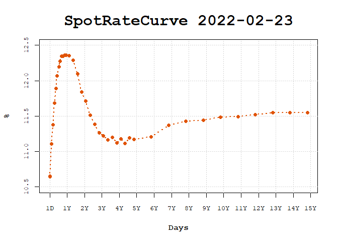
For another date.
curve <- get_curve_from_web("2011-02-23")
plot(curve)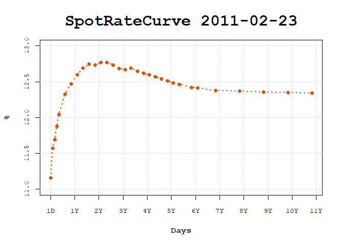
It can show the forward rates for the short term by selecting the first two years.
curve <- get_curve_from_web("2022-02-23")
plot(fixedincome::first(curve, "2 years"), show_forward = TRUE)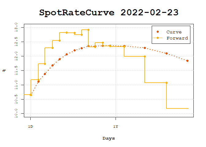
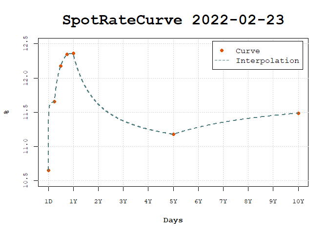
Once interpolation is set, it can be used in the plot.
curve_2y <- fixedincome::first(curve, "2 years")
interpolation(curve_2y) <- interp_flatforward()
plot(curve_2y, use_interpolation = TRUE, legend_location = "bottomright")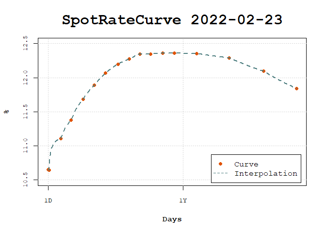
Parametric models like the Nelson-Siegel-Svensson model can be fitted to the curve.
beta1 <- as.numeric(fixedincome::last(curve, "1 day"))
beta2 <- as.numeric(curve[1]) - beta1
interpolation(curve) <- fit_interpolation(
  interp_nelsonsiegelsvensson(beta1, beta2, 0.01, 0.01, 2, 1), curve
)

interpolation(curve)
#> <Interpolation: nelsonsiegelsvensson >
#>  Parameters:
#>   beta1   beta2   beta3   beta4 lambda1 lambda2
#>   0.119  -0.013   1.000  -0.975   1.195   1.122
Once set to the curve it is used in the plot to show daily forward rates.
plot(curve, use_interpolation = TRUE, show_forward = TRUE, legend_location = "bottom")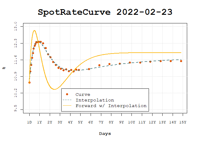
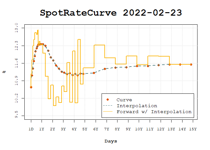
The interpolation can be changed in order to compare different interpolations and the effects in forward rates.
interpolation(curve) <- interp_flatforward()
plot(
  curve,
  use_interpolation = TRUE, show_forward = TRUE,
  legend_location = "bottomright"
)
Interpolation enables the creation of standardized curves, commonly used in risk management to build risk factors.
risk_terms <- c(1, c(3, 6, 9) * 21, c(1, 5, 10) * 252)
risk_curve <- curve[[risk_terms]]
interpolation(risk_curve) <- interp_flatforward()
plot(risk_curve, use_interpolation = TRUE)