
![]()
![]()
![]()
The goal of {equatiomatic} is to reduce the pain associated with writing LaTeX code from a fitted model. The package aims to support any model supported by {broom}. See the introduction to equatiomatic for currently supported models.
Install from CRAN with:
install.packages("equatiomatic")Or get the development version from GitHub with:
remotes::install_github("datalorax/equatiomatic")
The gif above shows the basic functionality.
To convert a model to LaTeX, feed a model object to
extract_eq():
library(equatiomatic)

# Fit a simple model
mod1 <- lm(mpg ~ cyl + disp, data = mtcars)

# Give the results to extract_eq
extract_eq(mod1)
#> $$
#> \operatorname{mpg} = \alpha + \beta_{1}(\operatorname{cyl}) + \beta_{2}(\operatorname{disp}) + \epsilon
#> $$\[\operatorname{mpg} = \alpha + \beta_{1}(\operatorname{cyl}) + \beta_{2}(\operatorname{disp}) + \epsilon\]
The model can be built in any standard way. It can handle shortcut syntax:
mod2 <- lm(mpg ~ ., data = mtcars)
extract_eq(mod2)
#> $$
#> \operatorname{mpg} = \alpha + \beta_{1}(\operatorname{cyl}) + \beta_{2}(\operatorname{disp}) + \beta_{3}(\operatorname{hp}) + \beta_{4}(\operatorname{drat}) + \beta_{5}(\operatorname{wt}) + \beta_{6}(\operatorname{qsec}) + \beta_{7}(\operatorname{vs}) + \beta_{8}(\operatorname{am}) + \beta_{9}(\operatorname{gear}) + \beta_{10}(\operatorname{carb}) + \epsilon
#> $$\[\operatorname{mpg} = \alpha + \beta_{1}(\operatorname{cyl}) + \beta_{2}(\operatorname{disp}) + \beta_{3}(\operatorname{hp}) + \beta_{4}(\operatorname{drat}) + \beta_{5}(\operatorname{wt}) + \beta_{6}(\operatorname{qsec}) + \beta_{7}(\operatorname{vs}) + \beta_{8}(\operatorname{am}) + \beta_{9}(\operatorname{gear}) + \beta_{10}(\operatorname{carb}) + \epsilon\]
When using categorical variables, it will include the levels of the variables as subscripts.
data("penguins", package = "equatiomatic")
mod3 <- lm(body_mass_g ~ bill_length_mm + species, data = penguins)
extract_eq(mod3)
#> $$
#> \operatorname{body\_mass\_g} = \alpha + \beta_{1}(\operatorname{bill\_length\_mm}) + \beta_{2}(\operatorname{species}_{\operatorname{Chinstrap}}) + \beta_{3}(\operatorname{species}_{\operatorname{Gentoo}}) + \epsilon
#> $$\[\operatorname{body\_mass\_g} = \alpha + \beta_{1}(\operatorname{bill\_length\_mm}) + \beta_{2}(\operatorname{species}_{\operatorname{Chinstrap}}) + \beta_{3}(\operatorname{species}_{\operatorname{Gentoo}}) + \epsilon\]
It helpfully preserves the order the variables are supplied in the formula:
set.seed(8675309)
d <- data.frame(cat1  = rep(letters[1:3], 100),
                cat2  = rep(LETTERS[1:3], each = 100),
                cont1 = rnorm(300, 100, 1),
                cont2 = rnorm(300, 50, 5),
                out   = rnorm(300, 10, 0.5))
mod4 <- lm(out ~ cont1 + cat2 + cont2 + cat1, data = d)
extract_eq(mod4)
#> $$
#> \operatorname{out} = \alpha + \beta_{1}(\operatorname{cont1}) + \beta_{2}(\operatorname{cat2}_{\operatorname{B}}) + \beta_{3}(\operatorname{cat2}_{\operatorname{C}}) + \beta_{4}(\operatorname{cont2}) + \beta_{5}(\operatorname{cat1}_{\operatorname{b}}) + \beta_{6}(\operatorname{cat1}_{\operatorname{c}}) + \epsilon
#> $$\[\operatorname{out} = \alpha + \beta_{1}(\operatorname{cont1}) + \beta_{2}(\operatorname{cat2}_{\operatorname{B}}) + \beta_{3}(\operatorname{cat2}_{\operatorname{C}}) + \beta_{4}(\operatorname{cont2}) + \beta_{5}(\operatorname{cat1}_{\operatorname{b}}) + \beta_{6}(\operatorname{cat1}_{\operatorname{c}}) + \epsilon\]
You can wrap the equations so that a specified number of terms appear
on the right-hand side of the equation using terms_per_line
(defaults to 4):
extract_eq(mod2, wrap = TRUE)#> $$
#> \begin{aligned}
#> \operatorname{mpg} &= \alpha + \beta_{1}(\operatorname{cyl}) + \beta_{2}(\operatorname{disp}) + \beta_{3}(\operatorname{hp})\ + \\
#> &\quad \beta_{4}(\operatorname{drat}) + \beta_{5}(\operatorname{wt}) + \beta_{6}(\operatorname{qsec}) + \beta_{7}(\operatorname{vs})\ + \\
#> &\quad \beta_{8}(\operatorname{am}) + \beta_{9}(\operatorname{gear}) + \beta_{10}(\operatorname{carb}) + \epsilon
#> \end{aligned}
#> $$\[\begin{aligned} \operatorname{mpg} &= \alpha + \beta_{1}(\operatorname{cyl}) + \beta_{2}(\operatorname{disp}) + \beta_{3}(\operatorname{hp})\ + \\ &\quad \beta_{4}(\operatorname{drat}) + \beta_{5}(\operatorname{wt}) + \beta_{6}(\operatorname{qsec}) + \beta_{7}(\operatorname{vs})\ + \\ &\quad \beta_{8}(\operatorname{am}) + \beta_{9}(\operatorname{gear}) + \beta_{10}(\operatorname{carb}) + \epsilon \end{aligned}\]
extract_eq(mod2, wrap = TRUE, terms_per_line = 6)#> $$
#> \begin{aligned}
#> \operatorname{mpg} &= \alpha + \beta_{1}(\operatorname{cyl}) + \beta_{2}(\operatorname{disp}) + \beta_{3}(\operatorname{hp}) + \beta_{4}(\operatorname{drat}) + \beta_{5}(\operatorname{wt})\ + \\
#> &\quad \beta_{6}(\operatorname{qsec}) + \beta_{7}(\operatorname{vs}) + \beta_{8}(\operatorname{am}) + \beta_{9}(\operatorname{gear}) + \beta_{10}(\operatorname{carb}) + \epsilon
#> \end{aligned}
#> $$\[\begin{aligned} \operatorname{mpg} &= \alpha + \beta_{1}(\operatorname{cyl}) + \beta_{2}(\operatorname{disp}) + \beta_{3}(\operatorname{hp}) + \beta_{4}(\operatorname{drat}) + \beta_{5}(\operatorname{wt})\ + \\ &\quad \beta_{6}(\operatorname{qsec}) + \beta_{7}(\operatorname{vs}) + \beta_{8}(\operatorname{am}) + \beta_{9}(\operatorname{gear}) + \beta_{10}(\operatorname{carb}) + \epsilon \end{aligned}\]
When wrapping, you can change whether the lines end with trailing
math operators like + (the default), or if they should
begin with them using operator_location = "end" or
operator_location = "start":
extract_eq(mod2, wrap = TRUE, terms_per_line = 4, operator_location = "start")#> $$
#> \begin{aligned}
#> \operatorname{mpg} &= \alpha + \beta_{1}(\operatorname{cyl}) + \beta_{2}(\operatorname{disp}) + \beta_{3}(\operatorname{hp})\\
#> &\quad + \beta_{4}(\operatorname{drat}) + \beta_{5}(\operatorname{wt}) + \beta_{6}(\operatorname{qsec}) + \beta_{7}(\operatorname{vs})\\
#> &\quad + \beta_{8}(\operatorname{am}) + \beta_{9}(\operatorname{gear}) + \beta_{10}(\operatorname{carb}) + \epsilon
#> \end{aligned}
#> $$\[\begin{aligned} \operatorname{mpg} &= \alpha + \beta_{1}(\operatorname{cyl}) + \beta_{2}(\operatorname{disp}) + \beta_{3}(\operatorname{hp})\\ &\quad + \beta_{4}(\operatorname{drat}) + \beta_{5}(\operatorname{wt}) + \beta_{6}(\operatorname{qsec}) + \beta_{7}(\operatorname{vs})\\ &\quad + \beta_{8}(\operatorname{am}) + \beta_{9}(\operatorname{gear}) + \beta_{10}(\operatorname{carb}) + \epsilon \end{aligned}\]
By default, all text in the equation is wrapped in
\operatorname{}. You can optionally have the variables
themselves be italicized (i.e. not be wrapped in
\operatorname{}) with ital_vars = TRUE:
extract_eq(mod2, wrap = TRUE, ital_vars = TRUE)#> $$
#> \begin{aligned}
#> mpg &= \alpha + \beta_{1}(cyl) + \beta_{2}(disp) + \beta_{3}(hp)\ + \\
#> &\quad \beta_{4}(drat) + \beta_{5}(wt) + \beta_{6}(qsec) + \beta_{7}(vs)\ + \\
#> &\quad \beta_{8}(am) + \beta_{9}(gear) + \beta_{10}(carb) + \epsilon
#> \end{aligned}
#> $$\[\begin{aligned} mpg &= \alpha + \beta_{1}(cyl) + \beta_{2}(disp) + \beta_{3}(hp)\ + \\ &\quad \beta_{4}(drat) + \beta_{5}(wt) + \beta_{6}(qsec) + \beta_{7}(vs)\ + \\ &\quad \beta_{8}(am) + \beta_{9}(gear) + \beta_{10}(carb) + \epsilon \end{aligned}\]
If you include extract_eq() in an R Markdown chunk,
{knitr} will render the equation. If you’d like to see the LaTeX code
wrap the call in print().
You can also use the preview_eq() function to preview
the equation in RStudio:
preview_eq(mod1)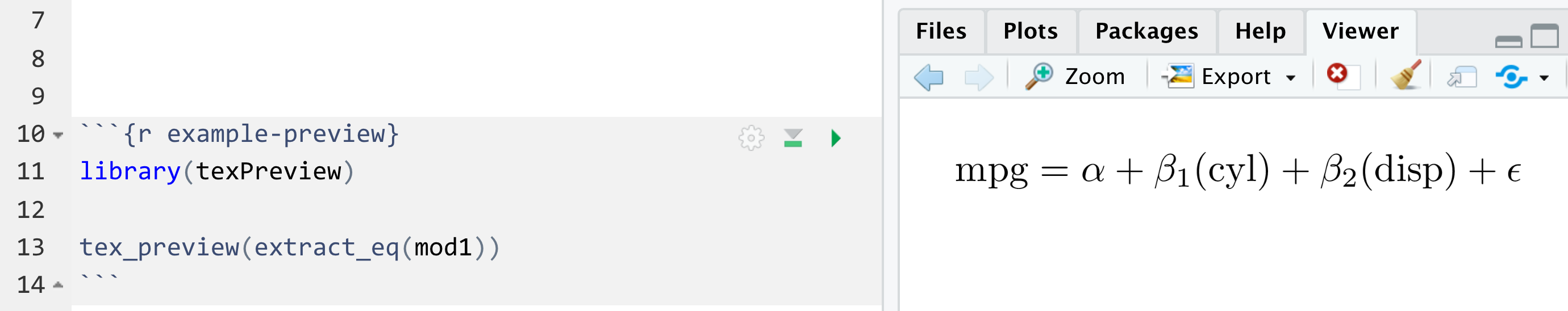
Both extract_eq() and preview_eq() work
with base R or {magrittr} pipes, so you can do something like this:
#library(magrittr)  # if you want to use %>% instead of |>

extract_eq(mod1) |>
  preview_eq()
# Or simply: preview_eq(mod1)There are several extra options you can enable with additional
arguments to extract_eq().
You can return actual numeric coefficients instead of Greek letters
with use_coefs = TRUE:
extract_eq(mod1, use_coefs = TRUE)#> $$
#> \operatorname{\widehat{mpg}} = 34.66 - 1.59(\operatorname{cyl}) - 0.02(\operatorname{disp})
#> $$\[\operatorname{\widehat{mpg}} = 34.66 - 1.59(\operatorname{cyl}) - 0.02(\operatorname{disp})\]
By default, it will remove doubled operators like “+ -”, but you can
keep those in (which is often useful for teaching) with
fix_signs = FALSE:
extract_eq(mod1, use_coefs = TRUE, fix_signs = FALSE)#> $$
#> \operatorname{\widehat{mpg}} = 34.66 + -1.59(\operatorname{cyl}) + -0.02(\operatorname{disp})
#> $$\[\operatorname{\widehat{mpg}} = 34.66 + -1.59(\operatorname{cyl}) + -0.02(\operatorname{disp})\]
This works in longer wrapped equations:
extract_eq(mod2, wrap = TRUE, terms_per_line = 3, use_coefs = TRUE,
  fix_signs = FALSE)
#> $$
#> \begin{aligned}
#> \operatorname{\widehat{mpg}} &= 12.3 + -0.11(\operatorname{cyl}) + 0.01(\operatorname{disp})\ + \\
#> &\quad -0.02(\operatorname{hp}) + 0.79(\operatorname{drat}) + -3.72(\operatorname{wt})\ + \\
#> &\quad 0.82(\operatorname{qsec}) + 0.32(\operatorname{vs}) + 2.52(\operatorname{am})\ + \\
#> &\quad 0.66(\operatorname{gear}) + -0.2(\operatorname{carb})
#> \end{aligned}
#> $$\[\begin{aligned} \operatorname{\widehat{mpg}} &= 12.3 + -0.11(\operatorname{cyl}) + 0.01(\operatorname{disp})\ + \\ &\quad -0.02(\operatorname{hp}) + 0.79(\operatorname{drat}) + -3.72(\operatorname{wt})\ + \\ &\quad 0.82(\operatorname{qsec}) + 0.32(\operatorname{vs}) + 2.52(\operatorname{am})\ + \\ &\quad 0.66(\operatorname{gear}) + -0.2(\operatorname{carb}) \end{aligned}\]
lm()You’re not limited to just lm models! {equatiomatic}
supports many other models, including logistic regression, probit
regression, and ordered logistic regression (with
MASS::polr()).
glm()model_logit <- glm(sex ~ bill_length_mm + species, data = penguins,
family = binomial(link = "logit"))
extract_eq(model_logit, wrap = TRUE, terms_per_line = 3)#> $$
#> \begin{aligned}
#> \log\left[ \frac { P( \operatorname{sex} = \operatorname{male} ) }{ 1 - P( \operatorname{sex} = \operatorname{male} ) } \right] &= \alpha + \beta_{1}(\operatorname{bill\_length\_mm}) + \beta_{2}(\operatorname{species}_{\operatorname{Chinstrap}})\ + \\
#> &\quad \beta_{3}(\operatorname{species}_{\operatorname{Gentoo}})
#> \end{aligned}
#> $$\[\begin{aligned} \log\left[ \frac { P( \operatorname{sex} = \operatorname{male} ) }{ 1 - P( \operatorname{sex} = \operatorname{male} ) } \right] &= \alpha + \beta_{1}(\operatorname{bill\_length\_mm}) + \beta_{2}(\operatorname{species}_{\operatorname{Chinstrap}})\ + \\ &\quad \beta_{3}(\operatorname{species}_{\operatorname{Gentoo}}) \end{aligned}\]
glm()model_probit <- glm(sex ~ bill_length_mm + species, data = penguins,
family = binomial(link = "probit"))
extract_eq(model_probit, wrap = TRUE, terms_per_line = 3)#> $$
#> \begin{aligned}
#> P( \operatorname{sex} = \operatorname{male} ) &= \Phi[\alpha + \beta_{1}(\operatorname{bill\_length\_mm}) + \beta_{2}(\operatorname{species}_{\operatorname{Chinstrap}})\ + \\
#> &\qquad\ \beta_{3}(\operatorname{species}_{\operatorname{Gentoo}})]
#> \end{aligned}
#> $$\[\begin{aligned} P( \operatorname{sex} = \operatorname{male} ) &= \Phi[\alpha + \beta_{1}(\operatorname{bill\_length\_mm}) + \beta_{2}(\operatorname{species}_{\operatorname{Chinstrap}})\ + \\ &\qquad\ \beta_{3}(\operatorname{species}_{\operatorname{Gentoo}})] \end{aligned}\]
MASS::polr()set.seed(1234)
df <- data.frame(
outcome = ordered(rep(LETTERS[1:3], 100), levels = LETTERS[1:3]),
continuous_1 = rnorm(300, 100, 1),
continuous_2 = rnorm(300, 50, 5))
model_ologit <- MASS::polr(outcome ~ continuous_1 + continuous_2,
data = df, Hess = TRUE, method = "logistic")
model_oprobit <- MASS::polr(outcome ~ continuous_1 + continuous_2,
data = df, Hess = TRUE, method = "probit")
extract_eq(model_ologit, wrap = TRUE)#> $$
#> \begin{aligned}
#> \log\left[ \frac { P( \operatorname{outcome} \leq \operatorname{A} ) }{ 1 - P( \operatorname{outcome} \leq \operatorname{A} ) } \right] &= \alpha_{1} + \beta_{1}(\operatorname{continuous\_1}) + \beta_{2}(\operatorname{continuous\_2}) \\
#> \log\left[ \frac { P( \operatorname{outcome} \leq \operatorname{B} ) }{ 1 - P( \operatorname{outcome} \leq \operatorname{B} ) } \right] &= \alpha_{2} + \beta_{1}(\operatorname{continuous\_1}) + \beta_{2}(\operatorname{continuous\_2})
#> \end{aligned}
#> $$\[\begin{aligned} \log\left[ \frac { P( \operatorname{outcome} \leq \operatorname{A} ) }{ 1 - P( \operatorname{outcome} \leq \operatorname{A} ) } \right] &= \alpha_{1} + \beta_{1}(\operatorname{continuous\_1}) + \beta_{2}(\operatorname{continuous\_2}) \\ \log\left[ \frac { P( \operatorname{outcome} \leq \operatorname{B} ) }{ 1 - P( \operatorname{outcome} \leq \operatorname{B} ) } \right] &= \alpha_{2} + \beta_{1}(\operatorname{continuous\_1}) + \beta_{2}(\operatorname{continuous\_2}) \end{aligned}\]
extract_eq(model_oprobit, wrap = TRUE)#> $$
#> \begin{aligned}
#> P( \operatorname{outcome} \leq \operatorname{A} ) &= \Phi[\alpha_{1} + \beta_{1}(\operatorname{continuous\_1}) + \beta_{2}(\operatorname{continuous\_2})] \\
#> P( \operatorname{outcome} \leq \operatorname{B} ) &= \Phi[\alpha_{2} + \beta_{1}(\operatorname{continuous\_1}) + \beta_{2}(\operatorname{continuous\_2})]
#> \end{aligned}
#> $$\[\begin{aligned} P( \operatorname{outcome} \leq \operatorname{A} ) &= \Phi[\alpha_{1} + \beta_{1}(\operatorname{continuous\_1}) + \beta_{2}(\operatorname{continuous\_2})] \\ P( \operatorname{outcome} \leq \operatorname{B} ) &= \Phi[\alpha_{2} + \beta_{1}(\operatorname{continuous\_1}) + \beta_{2}(\operatorname{continuous\_2})] \end{aligned}\]
ordinal::clm()set.seed(1234)
df <- data.frame(
outcome = ordered(rep(LETTERS[1:3], 100), levels = LETTERS[1:3]),
continuous_1 = rnorm(300, 1, 1),
continuous_2 = rnorm(300, 5, 5))
model_ologit <- ordinal::clm(outcome ~ continuous_1 + continuous_2,
data = df, link = "logit")
model_oprobit <- ordinal::clm(outcome ~ continuous_1 + continuous_2,
data = df, link = "probit")
extract_eq(model_ologit, wrap = TRUE)#> $$
#> \begin{aligned}
#> \log\left[ \frac { P( \operatorname{outcome} \leq \operatorname{A} ) }{ 1 - P( \operatorname{outcome} \leq \operatorname{A} ) } \right] &= \alpha_{1} + \beta_{1}(\operatorname{continuous\_1}) + \beta_{2}(\operatorname{continuous\_2}) \\
#> \log\left[ \frac { P( \operatorname{outcome} \leq \operatorname{B} ) }{ 1 - P( \operatorname{outcome} \leq \operatorname{B} ) } \right] &= \alpha_{2} + \beta_{1}(\operatorname{continuous\_1}) + \beta_{2}(\operatorname{continuous\_2})
#> \end{aligned}
#> $$\[\begin{aligned} \log\left[ \frac { P( \operatorname{outcome} \leq \operatorname{A} ) }{ 1 - P( \operatorname{outcome} \leq \operatorname{A} ) } \right] &= \alpha_{1} + \beta_{1}(\operatorname{continuous\_1}) + \beta_{2}(\operatorname{continuous\_2}) \\ \log\left[ \frac { P( \operatorname{outcome} \leq \operatorname{B} ) }{ 1 - P( \operatorname{outcome} \leq \operatorname{B} ) } \right] &= \alpha_{2} + \beta_{1}(\operatorname{continuous\_1}) + \beta_{2}(\operatorname{continuous\_2}) \end{aligned}\]
extract_eq(model_oprobit, wrap = TRUE)#> $$
#> \begin{aligned}
#> P( \operatorname{outcome} \leq \operatorname{A} ) &= \Phi[\alpha_{1} + \beta_{1}(\operatorname{continuous\_1}) + \beta_{2}(\operatorname{continuous\_2})] \\
#> P( \operatorname{outcome} \leq \operatorname{B} ) &= \Phi[\alpha_{2} + \beta_{1}(\operatorname{continuous\_1}) + \beta_{2}(\operatorname{continuous\_2})]
#> \end{aligned}
#> $$\[\begin{aligned} P( \operatorname{outcome} \leq \operatorname{A} ) &= \Phi[\alpha_{1} + \beta_{1}(\operatorname{continuous\_1}) + \beta_{2}(\operatorname{continuous\_2})] \\ P( \operatorname{outcome} \leq \operatorname{B} ) &= \Phi[\alpha_{2} + \beta_{1}(\operatorname{continuous\_1}) + \beta_{2}(\operatorname{continuous\_2})] \end{aligned}\]
If you would like to contribute to this package, we’d love your help! We are particularly interested in extending to more models. We hope to support any model supported by {broom} in the future.
Please note that the ‘equatiomatic’ project is released with a Contributor Code of Conduct. By contributing to this project, you agree to abide by its terms.
We’d like to thank the authors of the {palmerpenguins}
dataset for generously allowing us to incorporate the
penguins dataset in our package for example usage.
Horst AM, Hill AP, Gorman KB (2020). palmerpenguins: Palmer Archipelago (Antarctica) penguin data. R package version 0.1.0. https://allisonhorst.github.io/palmerpenguins/