The EAT algorithm performs a regression tree based on
CART methodology under a new approach that guarantees obtaining a
frontier as estimator that fulfills the property of free disposability.
This new technique has been baptized as Efficiency Analysis Trees. Some
of its main functions are:
To create homogeneous groups of DMUs in terms of their inputs and to know for each of these groups, what is the maximum expected output.
To know which DMUs exercise best practices and which of them do not obtain a performance according to their resources level.
To know what variables are more relevant in obtaining efficient levels of output.
You can install the released version of eat from CRAN with:
install.packages("eat")And the development version from GitHub with:
devtools::install_github("MiriamEsteve/EAT")library(eat)
data("PISAindex")NBMC) and 1 output
(S_PISA)single_model <- EAT(data = PISAindex,
x = 15, # input
y = 3) # output
#> [conflicted] Will prefer dplyr::filter over any other packageEAT objectprint(single_model)#> [1] y: [ 551 ] || R: 11507.5 n(t): 72
#>
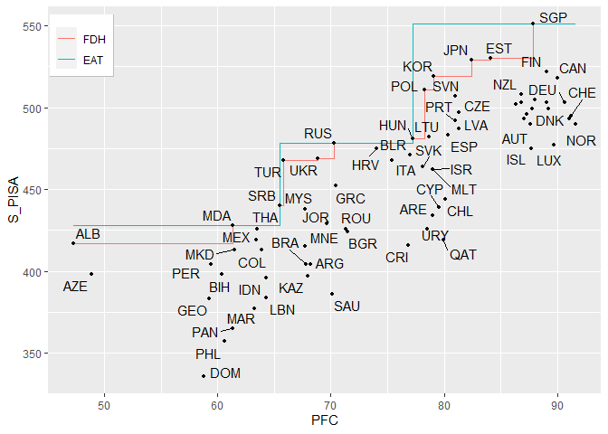
#> | [2] PFC < 77.2 --> y: [ 478 ] || R: 2324.47 n(t): 34
#>
#> | | [4] PFC < 65.45 --> y: [ 428 ] <*> || R: 390.17 n(t): 16
#>
#> | | [5] PFC >= 65.45 --> y: [ 478 ] <*> || R: 637.08 n(t): 18
#>
#> | [3] PFC >= 77.2 --> y: [ 551 ] <*> || R: 2452.83 n(t): 38
#>
#> <*> is a leaf nodeEAT objectsummary(single_model)#>
#> Formula: S_PISA ~ PFC
#>
#> # ========================== #
#> # Summary for leaf nodes #
#> # ========================== #
#>
#> id n(t) % S_PISA R(t)
#> 3 38 53 551 2452.83
#> 4 16 22 428 390.17
#> 5 18 25 478 637.08
#>
#> # ========================== #
#> # Tree #
#> # ========================== #
#>
#> Interior nodes: 2
#> Leaf nodes: 3
#> Total nodes: 5
#>
#> R(T): 3480.08
#> numStop: 5
#> fold: 5
#> max.depth:
#> max.leaves:
#>
#> # ========================== #
#> # Primary & surrogate splits #
#> # ========================== #
#>
#> Node 1 --> {2,3} || PFC --> {R: 4777.31, s: 77.2}
#>
#> Node 2 --> {4,5} || PFC --> {R: 1027.25, s: 65.45}EAT objectsize(single_model)#> The number of leaf nodes of the EAT model is: 3EAT objectfrontier.levels(single_model)#> The frontier levels of the outputs at the leaf nodes are:
#> S_PISA
#> 1 551
#> 2 428
#> 3 478EAT objectdescriptiveEAT <- descrEAT(single_model)
descriptiveEAT#> Node n(t) % mean var sd min Q1 median Q3 max RMSE
#> 1 1 72 100 455.06 2334.59 48.32 336 416.75 466.0 495.25 551 107.27
#> 2 2 34 47 416.88 1223.02 34.97 336 397.25 415.5 435.75 478 70.16
#> 3 3 38 53 489.21 851.95 29.19 419 478.00 494.0 504.50 551 68.17
#> 4 4 16 22 394.62 684.65 26.17 336 381.50 398.0 414.00 428 41.90
#> 5 5 18 25 436.67 889.29 29.82 386 415.25 433.5 468.00 478 50.48frontier(object = single_model,
FDH = TRUE,
observed.data = TRUE,
rwn = TRUE)#> Warning: ggrepel: 8 unlabeled data points (too many overlaps). Consider
#> increasing max.overlaps
multioutput <- EAT(data = PISAindex,
                   x = 6:18,
                   y = 3:5)
#> [conflicted] Removing existing preference
#> [conflicted] Will prefer dplyr::filter over any other package
#> Warning in preProcess(data = data, x = x, y = y, numStop = numStop, fold = fold, : Rows with NA values have been omitted .rankingEAT(object = multioutput,
barplot = TRUE,
threshold = 70,
digits = 2)#> $scores
#> Importance
#> AAE 100.00
#> WS 98.45
#> S 84.51
#> NBMC 83.37
#> HW 83.31
#> ABK 67.97
#> GDP_PPP 65.37
#> AIC 64.89
#> EQ 57.11
#> PR 57.05
#> I 57.05
#> PS 45.41
#> PFC 31.67
#>
#> $barplot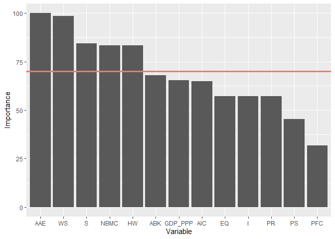
plotEAT(object = multioutput)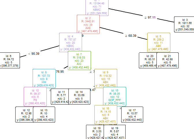
n <- nrow(PISAindex) # Observations in the dataset
t_index <- sample(1:n, n * 0.7) # Training indexes
training <- PISAindex[t_index, ] # Training set
test <- PISAindex[-t_index, ] # Test set

bestEAT(training = training,
        test = test,
        x = 6:18,
        y = 3:5,
        numStop = c(5, 7, 10),
        fold = c(5, 7))
#> Warning in preProcess(test, x, y, na.rm = na.rm): Rows with NA values have been omitted .
#> [conflicted] Removing existing preference

#> [conflicted] Will prefer dplyr::filter over any other package
#> [conflicted] Removing existing preference
#> [conflicted] Will prefer dplyr::filter over any other package
#> [conflicted] Removing existing preference
#> [conflicted] Will prefer dplyr::filter over any other package
#> [conflicted] Removing existing preference
#> [conflicted] Will prefer dplyr::filter over any other package
#> [conflicted] Removing existing preference
#> [conflicted] Will prefer dplyr::filter over any other package
#> [conflicted] Removing existing preference
#> [conflicted] Will prefer dplyr::filter over any other package
#> numStop fold RMSE leaves
#> 1 7 5 66.94 10
#> 2 7 7 66.94 10
#> 3 5 7 71.87 8
#> 4 5 5 84.60 7
#> 5 10 5 85.06 5
#> 6 10 7 85.06 5single_model <- EAT(data = PISAindex,
x = 15, # input
y = 3) # output#> [conflicted] Removing existing preference
#> [conflicted] Will prefer dplyr::filter over any other packagescores_EAT <- efficiencyEAT(data = PISAindex,
x = 15,
y = 3,
object = single_model,
scores_model = "BCC.OUT",
digits = 3,
FDH = TRUE)#> EAT_BCC_OUT FDH_BCC_OUT
#> SGP 1.000 1.000
#> JPN 1.042 1.000
#> KOR 1.062 1.000
#> EST 1.040 1.000
#> NLD 1.095 1.095
#> POL 1.078 1.000
#> CHE 1.113 1.113
#> CAN 1.064 1.064
#> DNK 1.118 1.118
#> SVN 1.087 1.024
#> BEL 1.104 1.062
#> FIN 1.056 1.056
#> SWE 1.104 1.104
#> GBR 1.091 1.091
#> NOR 1.124 1.124
#> DEU 1.095 1.095
#> IRL 1.111 1.069
#> AUT 1.124 1.082
#> CZE 1.109 1.044
#> LVA 1.131 1.066
#> FRA 1.118 1.075
#> ISL 1.160 1.116
#> NZL 1.085 1.043
#> PRT 1.120 1.055
#> AUS 1.095 1.054
#> RUS 1.000 1.000
#> ITA 1.021 1.021
#> SVK 1.187 1.037
#> LUX 1.155 1.155
#> HUN 1.146 1.000
#> LTU 1.143 1.060
#> ESP 1.141 1.075
#> USA 1.098 1.056
#> BLR 1.015 1.015
#> MLT 1.193 1.106
#> HRV 1.006 1.006
#> ISR 1.193 1.106
#> TUR 1.021 1.000
#> UKR 1.019 1.000
#> CYP 1.255 1.182
#> GRC 1.058 1.058
#> SRB 1.086 1.000
#> MYS 1.091 1.068
#> ALB 1.026 1.000
#> BGR 1.127 1.127
#> ARE 1.270 1.177
#> MNE 1.152 1.128
#> ROU 1.122 1.122
#> KAZ 1.204 1.179
#> MDA 1.000 1.000
#> AZE 1.075 1.048
#> THA 1.005 1.005
#> URY 1.293 1.200
#> CHL 1.241 1.169
#> QAT 1.315 1.239
#> MEX 1.021 1.021
#> BIH 1.075 1.048
#> CRI 1.149 1.149
#> JOR 1.114 1.093
#> PER 1.059 1.032
#> GEO 1.117 1.089
#> MKD 1.036 1.036
#> LBN 1.115 1.115
#> COL 1.036 1.036
#> BRA 1.183 1.158
#> ARG 1.183 1.158
#> IDN 1.081 1.081
#> SAU 1.238 1.215
#> MAR 1.135 1.135
#> PAN 1.173 1.173
#> PHL 1.199 1.168
#> DOM 1.274 1.241
#>
#> Model Mean Std. Dev. Min Q1 Median Q3 Max
#> EAT 1.114 0.074 1 1.061 1.110 1.110 1.315
#> FDH 1.081 0.065 1 1.030 1.069 1.069 1.241scores_CEAT <- efficiencyCEAT(data = PISAindex,
x = 15,
y = 3,
object = single_model,
scores_model = "BCC.INP",
digits = 3,
DEA = TRUE)#> CEAT_BCC_INP DEA_BCC_INP
#> SGP 0.878 1.000
#> JPN 0.872 0.986
#> KOR 0.878 0.989
#> EST 0.857 0.969
#> NLD 0.736 0.824
#> POL 0.862 0.968
#> CHE 0.697 0.777
#> CAN 0.768 0.865
#> DNK 0.693 0.772
#> SVN 0.821 0.920
#> BEL 0.735 0.821
#> FIN 0.787 0.888
#> SWE 0.724 0.809
#> GBR 0.750 0.840
#> NOR 0.680 0.757
#> DEU 0.723 0.809
#> IRL 0.731 0.816
#> AUT 0.712 0.792
#> CZE 0.788 0.880
#> LVA 0.758 0.843
#> FRA 0.725 0.808
#> ISL 0.669 0.739
#> NZL 0.769 0.862
#> PRT 0.776 0.865
#> AUS 0.754 0.845
#> RUS 0.846 0.936
#> ITA 0.756 0.832
#> SVK 0.717 0.787
#> LUX 0.660 0.729
#> HUN 0.779 0.864
#> LTU 0.768 0.851
#> ESP 0.755 0.838
#> USA 0.756 0.846
#> BLR 0.750 0.826
#> MLT 0.703 0.771
#> HRV 0.792 0.875
#> ISR 0.703 0.771
#> TUR 0.866 0.953
#> UKR 0.831 0.916
#> CYP 0.628 0.678
#> GRC 0.754 0.822
#> SRB 0.767 0.829
#> MYS 0.734 0.792
#> ALB 1.000 1.000
#> BGR 0.661 0.691
#> ARE 0.616 0.663
#> MNE 0.698 0.698
#> ROU 0.662 0.701
#> KAZ 0.696 0.696
#> MDA 0.771 0.825
#> AZE 0.967 0.967
#> THA 0.744 0.787
#> URY 0.602 0.637
#> CHL 0.638 0.692
#> QAT 0.591 0.599
#> MEX 0.746 0.755
#> BIH 0.782 0.782
#> CRI 0.615 0.615
#> JOR 0.682 0.731
#> PER 0.795 0.795
#> GEO 0.798 0.798
#> MKD 0.768 0.768
#> LBN 0.735 0.735
#> COL 0.739 0.739
#> BRA 0.697 0.697
#> ARG 0.693 0.693
#> IDN 0.735 0.735
#> SAU 0.674 0.674
#> MAR 0.748 0.748
#> PAN 0.770 0.770
#> PHL 0.780 0.780
#> DOM 0.804 0.804
#>
#> Model Mean Std. Dev. Min Q1 Median Q3 Max
#> CEAT 0.749 0.077 0.591 0.698 0.749 0.749 1
#> DEA 0.805 0.094 0.599 0.739 0.801 0.801 1efficiencyJitter(object = single_model,
df_scores = scores_EAT$EAT_BCC_OUT,
scores_model = "BCC.OUT",
lwb = 1.2)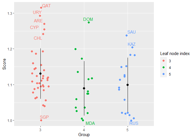
efficiencyDensity(df_scores = scores_EAT[, 3:4],
                  model = c("EAT", "FDH"))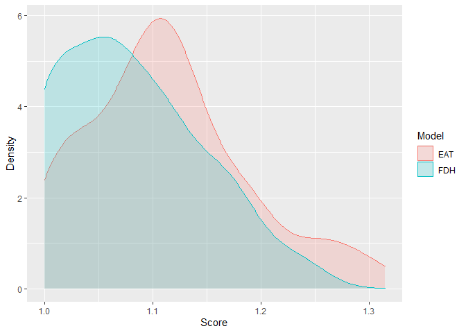
forest <- RFEAT(data = PISAindex,
                x = 6:18, # input
                y = 5, # output
                numStop = 5,
                m = 30,
                s_mtry = "BRM",
                na.rm = TRUE)
#> [conflicted] Removing existing preference
#> [conflicted] Will prefer dplyr::filter over any other packageRFEAT objectprint(forest)#>
#> Formula: M_PISA ~ NBMC + WS + S + PS + ABK + AIC + HW + EQ + PR + PFC + I + AAE + GDP_PPP
#>
#> # ========================== #
#> # Forest #
#> # ========================== #
#>
#> Error: 738.42
#> numStop: 5
#> No. of trees (m): 30
#> No. of inputs tried (s_mtry): BRMplotRFEAT(forest)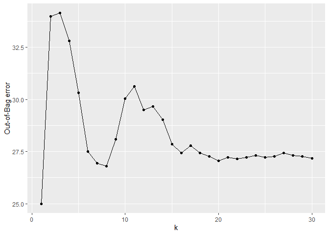
rankingRFEAT(object = forest, barplot = TRUE,
digits = 2)#> [conflicted] Removing existing preference
#> [conflicted] Will prefer dplyr::filter over any other package
#> [conflicted] Removing existing preference

#> [conflicted] Will prefer dplyr::filter over any other package
#> [conflicted] Removing existing preference
#> [conflicted] Will prefer dplyr::filter over any other package
#> [conflicted] Removing existing preference
#> [conflicted] Will prefer dplyr::filter over any other package
#> [conflicted] Removing existing preference
#> [conflicted] Will prefer dplyr::filter over any other package
#> [conflicted] Removing existing preference
#> [conflicted] Will prefer dplyr::filter over any other package
#> [conflicted] Removing existing preference
#> [conflicted] Will prefer dplyr::filter over any other package
#> [conflicted] Removing existing preference
#> [conflicted] Will prefer dplyr::filter over any other package
#> [conflicted] Removing existing preference
#> [conflicted] Will prefer dplyr::filter over any other package
#> [conflicted] Removing existing preference
#> [conflicted] Will prefer dplyr::filter over any other package
#> [conflicted] Removing existing preference
#> [conflicted] Will prefer dplyr::filter over any other package
#> [conflicted] Removing existing preference
#> [conflicted] Will prefer dplyr::filter over any other package
#> [conflicted] Removing existing preference
#> [conflicted] Will prefer dplyr::filter over any other package
#> $scores
#> Importance
#> PS 14.25
#> PR 14.08
#> AAE 13.97
#> EQ 11.86
#> S 10.80
#> HW 9.36
#> AIC 6.36
#> I 4.49
#> NBMC 3.26
#> WS -1.79
#> GDP_PPP -4.68
#> PFC -4.77
#> ABK -6.11
#>
#> $barplot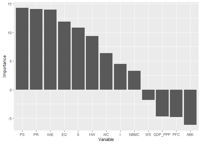
bestRFEAT(training = training,
          test = test,
          x = 6:18,
          y = 3:5,
          numStop = c(5, 10),
          m = c(30, 40),
          s_mtry = c("BRM", "3"))
#> Warning in preProcess(test, x, y, na.rm = na.rm): Rows with NA values have been omitted .
#> [conflicted] Removing existing preference
#> [conflicted] Will prefer dplyr::filter over any other package
#> [conflicted] Removing existing preference
#> [conflicted] Will prefer dplyr::filter over any other package
#> [conflicted] Removing existing preference
#> [conflicted] Will prefer dplyr::filter over any other package
#> [conflicted] Removing existing preference
#> [conflicted] Will prefer dplyr::filter over any other package
#> [conflicted] Removing existing preference
#> [conflicted] Will prefer dplyr::filter over any other package
#> [conflicted] Removing existing preference
#> [conflicted] Will prefer dplyr::filter over any other package
#> [conflicted] Removing existing preference
#> [conflicted] Will prefer dplyr::filter over any other package
#> [conflicted] Removing existing preference
#> [conflicted] Will prefer dplyr::filter over any other package
#> numStop m s_mtry RMSE
#> 1 5 40 3 57.44
#> 2 5 40 BRM 57.72
#> 3 5 30 BRM 58.39
#> 4 5 30 3 59.13
#> 5 10 30 BRM 62.43
#> 6 10 40 BRM 63.18
#> 7 10 40 3 65.02
#> 8 10 30 3 68.43efficiencyRFEAT(data = PISAindex,
x = 6:18, # input
y = 5, # output
object = forest,
FDH = TRUE)#> RFEAT_BCC_OUT FDH_BCC_OUT
#> SGP 0.936 1.000
#> JPN 1.024 1.000
#> KOR 1.004 1.000
#> EST 0.982 1.000
#> NLD 0.999 1.000
#> POL 0.982 1.000
#> CHE 1.026 1.002
#> CAN 1.010 1.008
#> DNK 1.017 1.014
#> SVN 1.004 1.000
#> BEL 1.006 1.000
#> FIN 1.021 1.018
#> SWE 1.029 1.028
#> GBR 1.019 1.000
#> NOR 1.039 1.030
#> DEU 1.028 1.032
#> IRL 1.031 1.032
#> AUT 1.024 1.034
#> CZE 1.014 1.000
#> LVA 0.997 1.000
#> FRA 1.037 1.000
#> ISL 1.070 1.042
#> NZL 1.048 1.045
#> PRT 0.995 1.000
#> AUS 1.054 1.051
#> RUS 0.963 1.000
#> ITA 1.011 1.000
#> SVK 0.997 1.000
#> LUX 1.053 1.000
#> HUN 1.008 1.000
#> LTU 1.020 1.000
#> ESP 1.030 1.000
#> USA 1.033 1.000
#> BLR 0.992 1.000
#> MLT 1.026 1.000
#> HRV 1.034 1.000
#> ISR 1.050 1.000
#> TUR 0.979 1.000
#> UKR 0.981 1.000
#> CYP 1.095 1.000
#> GRC 1.063 1.007
#> SRB 1.002 1.000
#> MYS 0.998 1.000
#> ALB 0.982 1.000
#> BGR 1.031 1.000
#> ARE 1.014 1.000
#> MNE 1.022 1.000
#> ROU 1.031 1.000
#> KAZ 1.018 1.000
#> MDA 1.003 1.000
#> AZE 0.972 1.000
#> THA 0.991 1.000
#> URY 1.045 1.000
#> CHL 1.097 1.005
#> QAT 1.070 1.000
#> MEX 1.005 1.000
#> BIH 1.042 1.000
#> CRI 1.085 1.000
#> JOR 1.046 1.000
#> PER 0.997 1.000
#> GEO 1.060 1.000
#> MKD 1.052 1.000
#> LBN 1.037 1.000
#> COL 1.055 1.000
#> BRA 1.074 1.000
#> ARG 1.157 1.000
#> IDN 1.034 1.000
#> SAU 1.100 1.000
#> MAR 1.031 1.000
#> PAN 1.116 1.000
#> PHL 1.049 1.000
#> DOM 1.145 1.000
#>
#> Model Mean Std. Dev. Min Q1 Median Q3 Max
#> RFEAT 1.029 0.039 0.936 1.003 1.026 1.026 1.157
#> FDH 1.005 0.012 1.000 1.000 1.000 1.000 1.051input <- c(6, 7, 8, 12, 17)
output <- 3:5
EAT_model <- EAT(data = PISAindex, x = input, y = output)#> [conflicted] Removing existing preference
#> [conflicted] Will prefer dplyr::filter over any other package
#> Warning in preProcess(data = data, x = x, y = y, numStop = numStop, fold = fold, : Rows with NA values have been omitted .RFEAT_model <- RFEAT(data = PISAindex, x = input, y = output)#> [conflicted] Removing existing preference
#> [conflicted] Will prefer dplyr::filter over any other package
#> Warning in preProcess(data = data, x = x, y = y, numStop = numStop, na.rm = na.rm): Rows with NA values have been omitted .# PREDICTIONS
predictions_EAT <- predict(object = EAT_model, newdata = PISAindex[, input])
predictions_RFEAT <- predict(object = RFEAT_model, newdata = PISAindex[, input])Please, check the vignette for more details.