![]()
![]()
![]()

Accurate documentation of a data pipeline is a first step to reproducibility, and a flow chart describing the steps taken to prepare data is a useful part of this documentation. In analyses that rely on data that is frequently updated, documenting a data flow by copying and pasting row counts into flowcharts in PowerPoint becomes quickly tedious. With interactive data analysis, and particularly using RMarkdown, code execution sometimes happens in a non-linear fashion, and this can lead to, at best, confusion and at worst erroneous analysis. Basing such documentation on what the code does when executed sequentially can be inaccurate when the data has being analysed interactively.
The goal of dtrackr is to take away this pain by
instrumenting and monitoring a dataframe through a dplyr
pipeline, creating a step-by-step summary of the important parts of the
wrangling as it actually happened to the dataframe, right into dataframe
metadata itself. This metadata can be used to generate documentation as
a flowchart, and allows both a quick overview of the data and also a
visual check of the actual data processing.
In general use dtrackr is expected to be installed
alongside the tidyverse set of packages. It is recommended
to install tidyverse first.
Binary packages of dtrackr are available on CRAN and
r-universe for macOS and Windows.
dtrackr can be installed from source on Linux.
dtrackr has been tested on R versions 3.6, 4.0, 4.1 and
4.2.
You can install the released version of dtrackr from CRAN with:
install.packages("dtrackr")For installation from source on Linux, dtrackr has
required transitive dependencies on a few system libraries. These can be
installed with the following commands:
# Ubuntu 20.04 and other debian based distributions:
sudo apt-get install libcurl4-openssl-dev libssl-dev librsvg2-dev \
  libicu-dev libnode-dev libpng-dev libjpeg-dev libpoppler-cpp-dev

# Centos 8
sudo dnf install libcurl-devel openssl-devel librsvg2-devel \
  libicu-devel libpng-devel libjpeg-turbo-devel poppler-devel

# for other linux distributions I suggest using the R pak library:
# install.packages("pak")
# pak::pkg_system_requirements("dtrackr")

# N.B. There are additional suggested R package dependencies on
# the `tidyverse` and `rstudioapi` packages which have a longer set of dependencies.
# We suggest you install them individually first if required.dtrackrEarly release versions are available on the r-universe.
This will typically be more up to date than CRAN.
# Enable repository from terminological
options(repos = c(
  terminological = 'https://terminological.r-universe.dev',
  CRAN = 'https://cloud.r-project.org'))
# Download and install dtrackr in R
install.packages('dtrackr')
The unstable development version is available from GitHub with:
# install.packages("devtools")
devtools::install_github("terminological/dtrackr")Suppose we are constructing a data set with out initial input being
the iris data. Our analysis depends on some
cutOff parameter and we want to prepare a stratified data
set that excludes flowers with narrow petals, and those with the biggest
petals of each Species. With dtrackr we can mix regular
dplyr commands with additional dtrackr
commands such as comment and status, and an
enhanced implementation of dplyr::filter, called
exclude_all, and include_any.
# a pipeline parameter
cutOff = 3

# the pipeline
dataset = iris %>%
  track() %>%
  status() %>%
  group_by(Species) %>%
  status(
    short = p_count_if(Sepal.Width<cutOff),
    long= p_count_if(Sepal.Width>=cutOff),
    .messages=c("consisting of {short} short sepal <{cutOff}","and {long} long sepal >={cutOff}")
  )  %>%
  exclude_all(
    Petal.Width<0.3 ~ "excluding {.excluded} with narrow petals",
    Petal.Width == max(Petal.Width) ~ "and {.excluded} outlier"
  ) %>%
  comment("test message") %>%
  status(.messages = "{.count} of type {Species}") %>%
  ungroup() %>%
  status(.messages = "{.count} together with cutOff {cutOff}")
Having prepared our dataset we conduct our analysis, and want to write it up and prepare it for submission. As a key part of documenting the data pipeline a visual summary is useful, and for bio-medical journals or clinical trials often a requirement.
dataset %>% flowchart()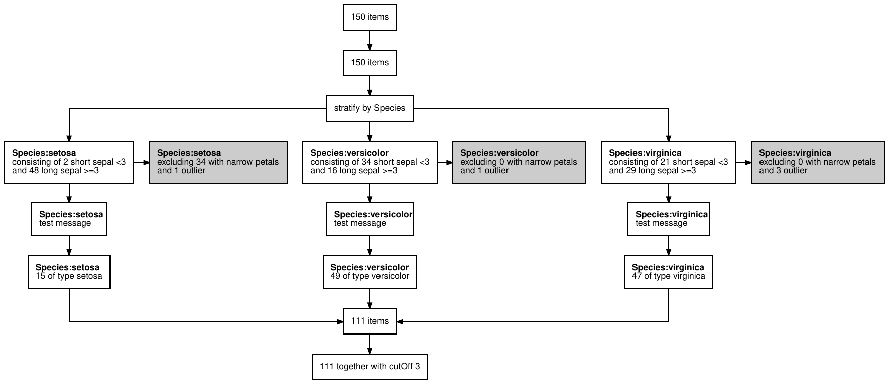
And your publication ready data pipeline, with any assumptions you
care to document, is creates in a format of your choice (as long as that
choice is one of pdf, png, svg or
ps), ready for submission to Nature.
This is a trivial example, but the more complex the pipeline, the bigger benefit you will get.
Check out the main documentation for more details, and in particular the getting started vignette.
The authors gratefully acknowledge the support of the UK Research and Innovation AI programme of the Engineering and Physical Sciences Research Council EPSRC grant EP/Y028392/1.