The goal of drpop is to provide users doubly robust and efficient estimates of population size and the confidence intervals for a capture-recapture problem.
You can install the released version of drpop from CRAN with:
install.packages("drpop")And the development version from GitHub with:
# install.packages("devtools")
devtools::install_github("mqnjqrid/drpop")This is a basic example which shows you how to solve a common problem:
library(drpop)
#> Registered S3 methods overwritten by 'tibble':
#> method from
#> format.tbl pillar
#> print.tbl pillar
n = 1000
x = matrix(rnorm(n*3, 2, 1), nrow = n)
expit = function(xi) {
exp(sum(xi))/(1 + exp(sum(xi)))
}
y1 = unlist(apply(x, 1, function(xi) {sample(c(0, 1), 1, replace = TRUE, prob = c(1 - expit(-0.6 + 0.4*xi), expit(-0.6 + 0.4*xi)))}))
y2 = unlist(apply(x, 1, function(xi) {sample(c(0, 1), 1, replace = TRUE, prob = c(1 - expit(-0.6 + 0.3*xi), expit(-0.6 + 0.3*xi)))}))
datacrc = cbind(y1, y2, exp(x/2))[y1+y2 > 0, ]
estim <- popsize(data = datacrc, func = c("gam"), nfolds = 2, K = 2)
#> Warning: package 'dplyr' was built under R version 4.0.5
#> Loading required package: tidyr
#> Loaded gam 1.20
#> Warning in popsize_base(data, K = K, j0 = j, k0 = k, filterrows = filterrows, :
#> Plug-in variance is not well-defined. Returning variance evaluated using DR
#> estimator formula
# The population size estimates are 'n' and the standard deviations are 'sigman'
print(estim)
#> listpair model method psi sigma n sigman cin.l cin.u
#> 1 1,2 gam DR 0.820 1.015 955 31.886 893 1018
#> 2 1,2 gam PI 0.810 1.015 967 32.150 904 1030
#> 3 1,2 gam TMLE 0.822 0.921 953 29.515 895 1010
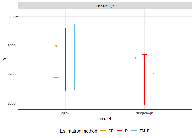
## basic example codeThe following shows the confidence interval of estimates for a toy data. Real population size is 3000.
library(drpop)

n = 3000
x = matrix(rnorm(n*3, 2,1), nrow = n)

expit = function(xi) {
  exp(sum(xi))/(1 + exp(sum(xi)))
}
y1 = unlist(apply(x, 1, function(xi) {sample(c(0, 1), 1, replace = TRUE, prob = c(1 - expit(-0.6 + 0.4*xi), expit(-0.6 + 0.4*xi)))}))
y2 = unlist(apply(x, 1, function(xi) {sample(c(0, 1), 1, replace = TRUE, prob = c(1 - expit(-0.6 + 0.3*xi), expit(-0.6 + 0.3*xi)))}))
datacrc = cbind(y1, y2, exp(x/2))[y1+y2>0,]

estim <- popsize(data = datacrc, func = c("gam", "rangerlogit"), nfolds = 2, margin = 0.01)
#> Warning in popsize_base(data, K = K, j0 = j, k0 = k, filterrows = filterrows, :
#> Plug-in variance is not well-defined. Returning variance evaluated using DR
#> estimator formula
print(estim)
#>   listpair       model method   psi sigma    n sigman cin.l cin.u
#> 1      1,2         gam     DR 0.794 1.001 2999 56.258  2889  3109
#> 2      1,2         gam     PI 0.807 1.001 2951 55.612  2842  3060
#> 3      1,2         gam   TMLE 0.805 1.059 2960 58.228  2846  3074
#> 4      1,2 rangerlogit     DR 0.806 0.764 2956 45.880  2866  3046
#> 5      1,2 rangerlogit     PI 0.827 0.764 2881 44.678  2794  2969
#> 6      1,2 rangerlogit   TMLE 0.821 0.841 2902 48.147  2807  2996
plotci(estim)
#> Warning: package 'ggplot2' was built under R version 4.0.4
#result = melt(as.data.frame(estim), variable.name = "estimator", value.name = "population_size")
#ggplot(result, aes(x = population_size - n, fill = estimator, color = estimator)) +
#  geom_density(alpha = 0.4) +
#  xlab("Bias on n")
The following shows confidence interval of estimates for toy data with a categorical covariate. Real population size is 10000.
library(drpop)
n = 10000
x = matrix(rnorm(n*3, 2, 1), nrow = n)
expit = function(xi) {
  exp(sum(xi))/(1 + exp(sum(xi)))
}
catcov = sample(c('m','f'), n, replace = TRUE, prob = c(0.45, 0.55))

y1 = unlist(apply(x, 1, function(xi) {sample(c(0, 1), 1, replace = TRUE, prob = c(1 - expit(-0.6 + 0.4*xi), expit(-0.6 + 0.4*xi)))}))
y2 = sapply(1:n, function(i) {sample(c(0, 1), 1, replace = TRUE, prob = c(1 - expit(-0.6 + 0.3*(catcov[i] == 'm') + 0.3*x[i,]), expit(-0.6 + 0.3*(catcov[i] == 'm') + 0.3*x[i,])))})
datacrc = cbind.data.frame(y1, y2, exp(x/2), catcov)[y1+y2>0,]

result = popsize_cond(data = datacrc, condvar = 'catcov')
#> Warning in popsize_base(data = datasub, K = K, filterrows = filterrows, : Plug-
#> in variance is not well-defined. Returning variance evaluated using DR estimator
#> formula

#> Warning in popsize_base(data = datasub, K = K, filterrows = filterrows, : Plug-
#> in variance is not well-defined. Returning variance evaluated using DR estimator
#> formula
fig = plotci(result)
fig + geom_hline(yintercept = table(catcov), color = "brown", linetype = "dashed")