![]()
![]()
![]()
![]()
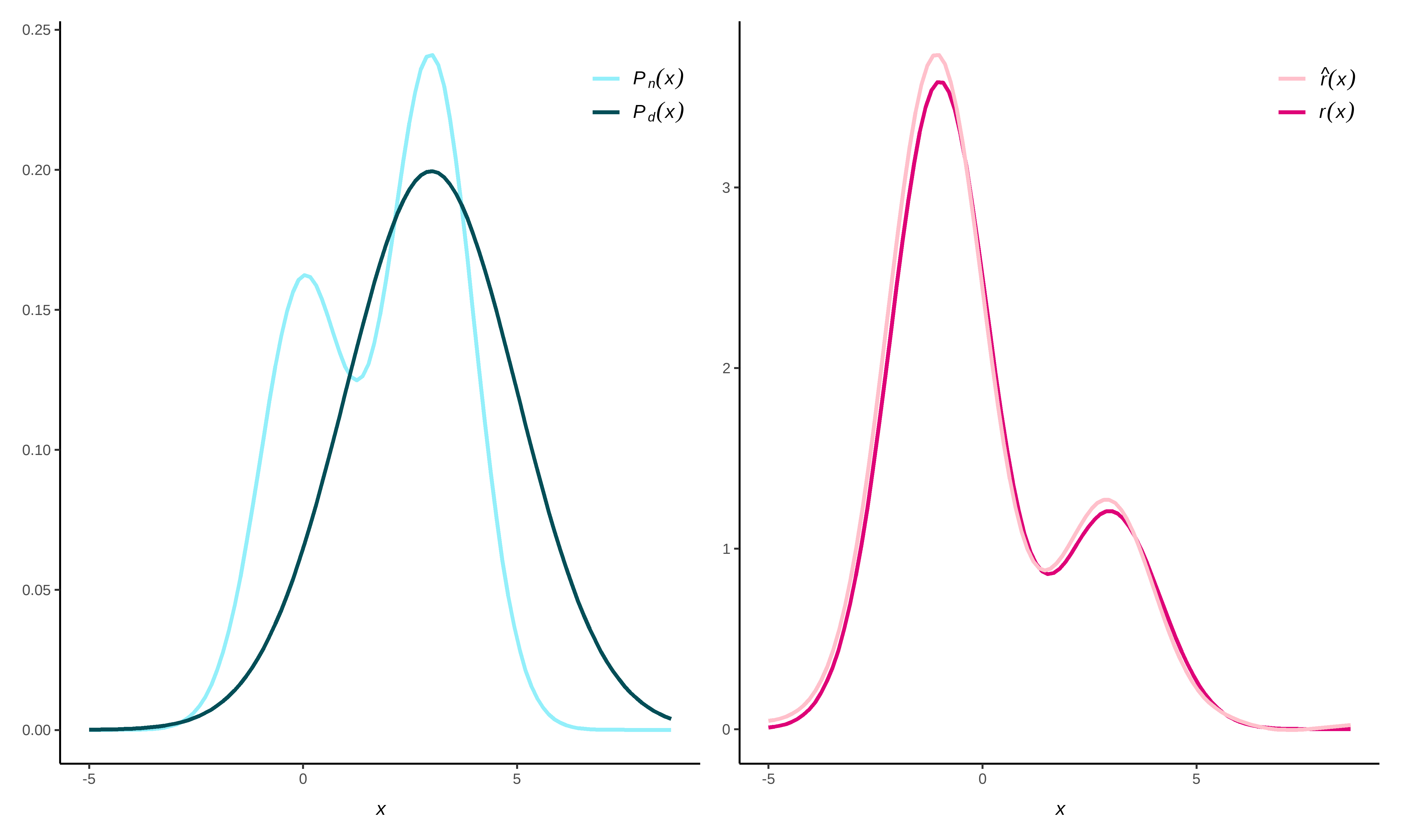
This package provides functionality to directly estimate a density ratio \[r(x) = \frac{p_\text{nu}(x)}{p_{\text{de}}(x)},\] without estimating the numerator and denominator density separately. Density ratio estimation serves many purposes, for example, prediction, outlier detection, change-point detection in time-series, importance weighting under domain adaptation (i.e., sample selection bias) and evaluation of synthetic data utility. The key idea is that differences between data distributions can be captured in their density ratio, which is estimated over the entire multivariate space of the data. Subsequently, the density ratio values can be used to summarize the dissimilarity between the two distributions in a discrepancy measure.
C++ using Rcpp and
RcppArmadillo.densityratio in practice).ulsif()), Kullback-Leibler importance estimation procedure
(kliep()), kernel mean matching (kmm()), ratio
of estimated densities (naive()), spectral density ratio
estimation (spectral() and least-squares
heterodistributional subspace search (lhss()).predict(), print() and summary()
functions for all density ratio estimation methods; built-in data sets
for quick testing.You can install the stable release of densityratio from
CRAN
with:
install.packages('densityratio')For the development version, use:
remotes::install_github("thomvolker/densityratio")The package contains several functions to estimate the density ratio
between the numerator data and the denominator data. To illustrate the
functionality, we make use of the in-built simulated data sets
numerator_data and denominator_data, that both
consist of the same five variables.
library(densityratio)

head(numerator_data)
#> # A tibble: 6 × 5
#>   x1    x2         x3     x4     x5
#>   <fct> <fct>   <dbl>  <dbl>  <dbl>
#> 1 A     G1    -0.0299  0.967 -1.26
#> 2 C     G1     2.29   -0.475  2.40
#> 3 A     G1     1.37    0.577 -0.172
#> 4 B     G2     1.44   -0.193 -0.708
#> 5 A     G1     1.01    2.23   2.01
#> 6 C     G2     1.83    0.762  3.71

fit <- ulsif(
  df_numerator = numerator_data$x5,
  df_denominator = denominator_data$x5,
  nsigma = 5,
  nlambda = 5
)

class(fit)
#> [1] "ulsif"
We can ask for the summary() of the estimated density
ratio object, that contains the optimal kernel weights (optimized using
cross-validation) and a measure of discrepancy between the numerator and
denominator densities.
summary(fit)
#>
#> Call:
#> ulsif(df_numerator = numerator_data$x5, df_denominator = denominator_data$x5,     nsigma = 5, nlambda = 5)
#>
#> Kernel Information:
#>   Kernel type: Gaussian with L2 norm distances
#>   Number of kernels: 200
#>
#> Optimal sigma: 0.3726142
#> Optimal lambda: 0.03162278
#> Optimal kernel weights: num [1:201] 0.43926 0.01016 0.00407 0.01563 0.01503 ...
#>
#> Pearson divergence between P(nu) and P(de): 0.2801
#> For a two-sample homogeneity test, use 'summary(x, test = TRUE)'.
To formally evaluate whether the numerator and denominator densities differ significantly, you can perform a two-sample homogeneity test as follows.
summary(fit, test = TRUE)
#>
#> Call:
#> ulsif(df_numerator = numerator_data$x5, df_denominator = denominator_data$x5,     nsigma = 5, nlambda = 5)
#>
#> Kernel Information:
#>   Kernel type: Gaussian with L2 norm distances
#>   Number of kernels: 200
#>
#> Optimal sigma: 0.3726142
#> Optimal lambda: 0.03162278
#> Optimal kernel weights: num [1:201] 0.43926 0.01016 0.00407 0.01563 0.01503 ...
#>
#> Pearson divergence between P(nu) and P(de): 0.2801
#> Pr(P(nu)=P(de)) < .001
#> Bonferroni-corrected for testing with r(x) = P(nu)/P(de) AND r*(x) = P(de)/P(nu).
The probability that numerator and denominator samples share a common data generating mechanism is very small.
The ulsif-object also contains the (hyper-)parameters
used in estimating the density ratio, such as the centers used in
constructing the Gaussian kernels (fit$centers), the
different bandwidth parameters (fit$sigma) and the
regularization parameters (fit$lambda). Using these
variables, we can obtain the estimated density ratio using
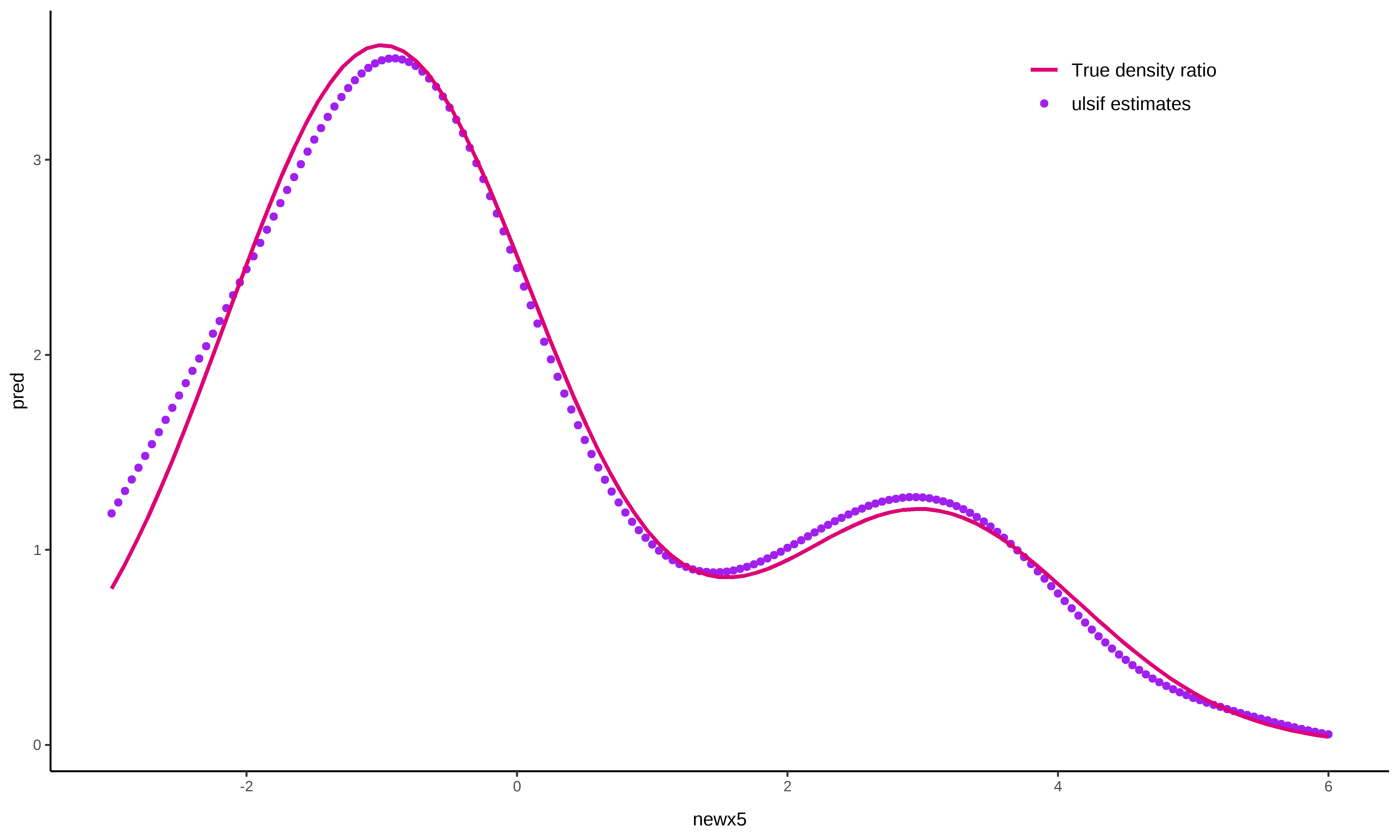
predict().
# obtain predictions for the numerator samples

newx5 <- seq(from = -3, to = 6, by = 0.05)
pred <- predict(fit, newdata = newx5)

ggplot() +
  geom_point(aes(x = newx5, y = pred, col = "ulsif estimates")) +
  stat_function(
    mapping = aes(col = "True density ratio"),
    fun = dratio,
    args = list(p = 0.4, dif = 3, mu = 3, sd = 2),
    linewidth = 1
  ) +
  theme_classic() +
  scale_color_manual(name = NULL, values = c("#de0277", "purple")) +
  theme(
    legend.position = "inside",
    legend.position.inside = c(0.8, 0.9),
    text = element_text(size = 50),
    legend.text = element_text(size = 50),
  )
By default, all functions in the densityratio package
standardize the data to the numerator means and standard deviations.
This is done to ensure that the importance of each variable in the
kernel estimates is not dependent on the scale of the data. By setting
scale = "denominator" one can scale the data to the means
and standard deviations of the denominator data, and by setting
scale = FALSE the data remains on the original scale.
All of the functions in the densityratio package accept
categorical variables types. However, note that internally, these
variables are one-hot encoded, which can lead to a high-dimensional
feature-space.
summary(numerator_data$x1)
#>   A   B   C
#> 351 339 310
summary(denominator_data$x1)
#>   A   B   C
#> 252 232 516

fit_cat <- ulsif(
  df_numerator = numerator_data$x1,
  df_denominator = denominator_data$x1
)
#> Warning in check.sigma(nsigma, sigma_quantile, sigma, dist_nu): There are duplicate values in 'sigma', only the unique values are used.

aggregate(
  predict(fit_cat) ~ numerator_data$x1,
  FUN = unique
)
#>   numerator_data$x1 predict(fit_cat)
#> 1                 A        1.3005360
#> 2                 B        1.3574809
#> 3                 C        0.6379142

table(numerator_data$x1) / table(denominator_data$x1)
#>
#>         A         B         C
#> 1.3928571 1.4612069 0.6007752
This transformation can give a reasonable estimate of the ratio of proportions in the different data sets (although there is some regularization applied such that the estimated odds are closer to one than seen in the real data).
After transforming all variables to numeric variables, it is possible to calculate the density ratio over the entire multivariate space of the data.
fit_all <- ulsif(
  df_numerator = numerator_data,
  df_denominator = denominator_data
)

summary(fit_all, test = TRUE, parallel = TRUE)
#>
#> Call:
#> ulsif(df_numerator = numerator_data, df_denominator = denominator_data)
#>
#> Kernel Information:
#>   Kernel type: Gaussian with L2 norm distances
#>   Number of kernels: 200
#>
#> Optimal sigma: 1.065369
#> Optimal lambda: 0.1623777
#> Optimal kernel weights: num [1:201] 0.5691 0.1511 0.0959 0.0118 0.0149 ...
#>
#> Pearson divergence between P(nu) and P(de): 0.4629
#> Pr(P(nu)=P(de)) < .001
#> Bonferroni-corrected for testing with r(x) = P(nu)/P(de) AND r*(x) = P(de)/P(nu).Besides ulsif(), the package contains several other
functions to estimate a density ratio.
naive() estimates the numerator and denominator
densities separately, and subsequently takes there ratio.kliep() estimates the density ratio directly through
the Kullback-Leibler importance estimation procedure.kmm() estimates the density ratio through kernel mean
matching.lhss() estimates the density ratio in a subspace where
the two distributions are most different using least-squares
heterodistributional subspace search.spectral() estimates the density ratio using a spectral
series approach.We display kliep() and naive() as examples
here. The other functions are discussed in the Get
Started vignette.
fit_naive <- naive(
  df_numerator = numerator_data$x5,
  df_denominator = denominator_data$x5
)

fit_kliep <- kliep(
  df_numerator = numerator_data$x5,
  df_denominator = denominator_data$x5
)


pred_naive <- predict(fit_naive, newdata = newx5)
pred_kliep <- predict(fit_kliep, newdata = newx5)


ggplot(data = NULL, aes(x = newx5)) +
  geom_point(aes(y = pred, col = "ulsif estimates")) +
  geom_point(aes(y = pred_naive, col = "naive estimates")) +
  geom_point(aes(y = pred_kliep, col = "kliep estimates")) +
  stat_function(aes(x = NULL, col = "True density ratio"),
    fun = dratio, args = list(p = 0.4, dif = 3, mu = 3, sd = 2),
    linewidth = 1
  ) +
  theme_classic() +
  scale_color_manual(name = NULL, values = c("pink", "#512970", "#de0277", "purple")) +
  theme(
    legend.position = "inside",
    legend.position.inside = c(0.8, 0.9),
    text = element_text(size = 50),
    legend.text = element_text(size = 50),
  )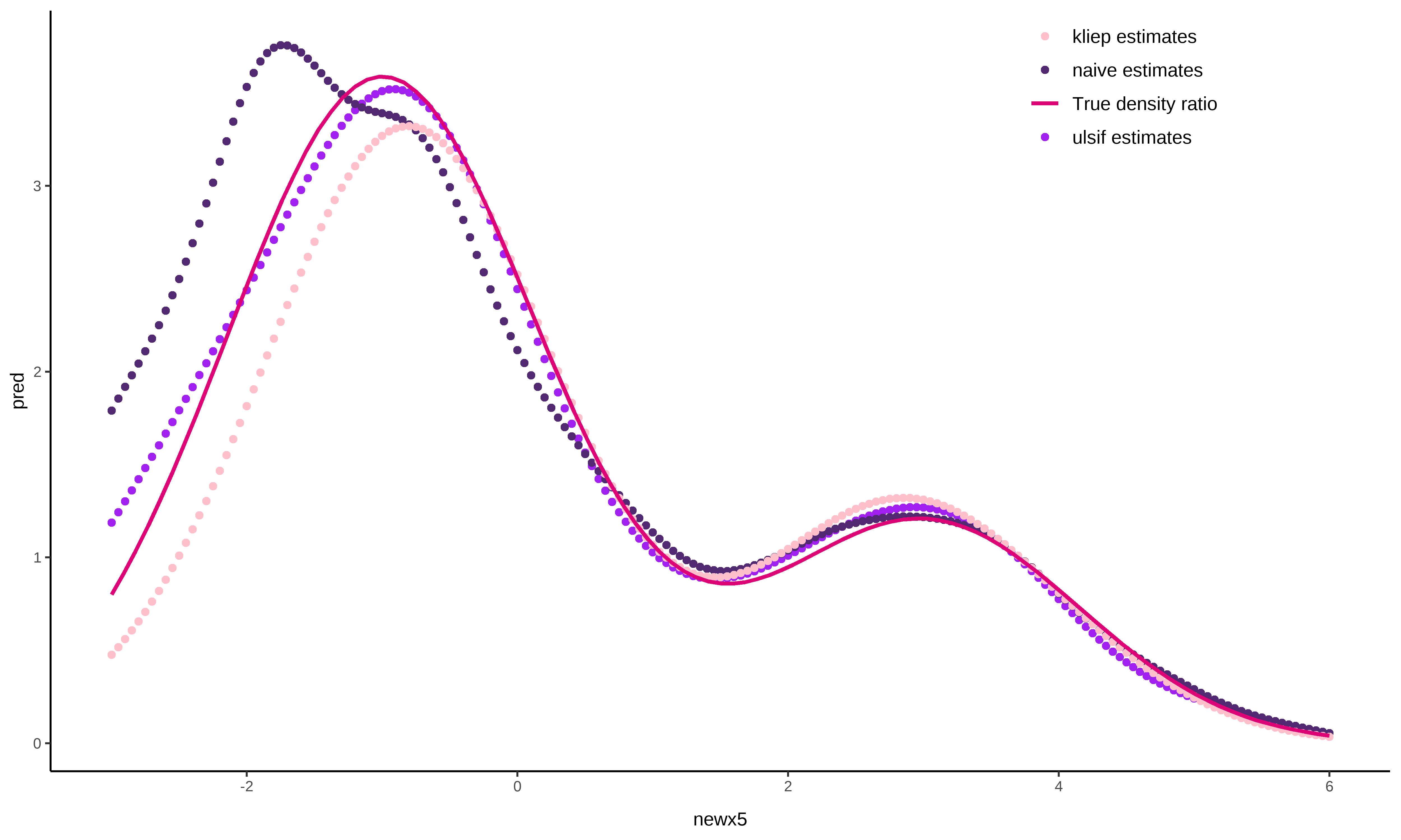
The figure directly shows that ulsif() and
kliep() come rather close to the true density ratio
function in this example, and outperform the naive()
solution.
This package is still in development, and I’ll be happy to take feedback and suggestions. Please submit these through GitHub Issues.
Books
Papers
Density ratio estimation for the evaluation of the utility of synthetic data: Volker, De Wolf and Van Kesteren (2023). Assessing the utility of synthetic data: A density ratio perspective
Density ratio estimation for covariate shift: Huang, Smola, Gretton, Borgwardt and Schölkopf (2007). Correcting sample selection bias by unlabeled data
High-dimensional density ratio estimation through a spectral series approach: Izbicki, Lee and Schafer (2014). High-dimensional density ratio estimation with extensions to approximate likelihood computation
Least-squares density ratio estimation: Sugiyama, Hido and Kanamori (2009). A least-squares approach to direct importance estimation
Volker, T.B., Poses, C. & Van Kesteren, E.J. (2023). densityratio: Distribution comparison through density ratio estimation. https://doi.org/10.5281/zenodo.8307818