## knitr settings
library(knitr)
opts_knit$set(root.dir=normalizePath('./'))
opts_chunk$set(fig.path = "./tools/README_fig/", dev='png')covafillr version can be installed from CRAN with
install.packages("covafillr")The development version of covafillr can be installed with
devtools::install_github("calbertsen/covafillr")To use covafillr with JAGS, JAGS
must be installed before the covafillr package, and the
package must be installed using the same compiler as JAGS is installed
with.
On Unix(-like) systems, pkg-config is used to find the
relevant paths to compile covafillr against
JAGS, such as
pkg-config --cflags jags
pkg-config --libs jags
## -I/usr/local/include/JAGS
## -L/usr/local/lib -ljagsThe package will only be installed with the JAGS module if the
configure argument --with-jags is given. Note that the
package must be compiled with the same compiler as
JAGS.
On Windows, the R package rjags is used to
find the paths. covafillr can be installed without using
rjags by setting a system variable JAGS_ROOT
to the folder where JAGS is installed, e.g., by running
Sys.setenv(JAGS_ROOT='C:/Program Files/JAGS/JAGS-4.1.0')before installation. Similar to Unix(-like) systems, the package is
only installed with the JAGS module if the system variable
USE_JAGS is set, e.g., by running
Sys.setenv(USE_JAGS='yes')Note that more examples are available in the inst/examples folder.
library(methods)
library(covafillr)
The package can be used from R to do local polynomial
regression and a search tree approximation of local polynomial
regression. Both are implemented with reference classes.
The reference class for local polynomial regression is called
covafill.
methods::getRefClass('covafill')## Generator for class "covafill":
##
## Class fields:
##
## Name: ptr
## Class: externalptr
## Locked Fields: "ptr"
##
##
## Class Methods:
## "import", "getDegree", ".objectParent", "setBandwith", "residuals",
## "usingMethods", "show", "getClass", "untrace", "export",
## "copy#envRefClass", "initialize", ".objectPackage", "callSuper",
## "getDim", "copy", "getBandwith", "predict", "initFields",
## "getRefClass", "trace", "field"
##
## Reference Superclasses:
## "envRefClass"To illustrate the usage we simulate data.
fn <- function(x) x ^ 4 - x ^ 2
x <- runif(2000,-10,10)
y <- fn(x) + rnorm(2000,0,0.1)
An object of the reference class is created by
cf <- covafill(coord = x,obs = y,p = 5L)where p is the polynomial degree. The bandwith can be set by the
argument h. By default, a value is suggested by the function
suggestBandwith. Information about the class can be
extracted (and changed) by the following functions:
cf$getDim()## [1] 1cf$getDegree()## [1] 5cf$getBandwith()## [1] 15.2975cf$setBandwith(1.0)## [1] 1cf$getBandwith()## [1] 1To do local polynomial regression at a point, the
$predict function is used.
x0 <- seq(-3,3,0.1)
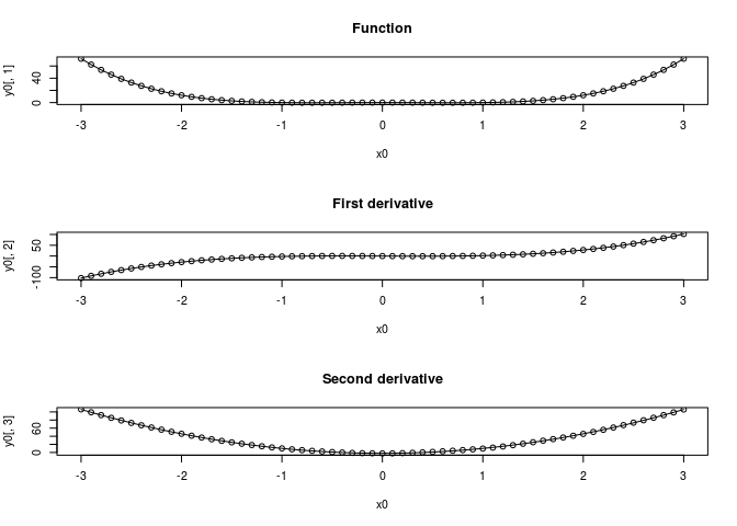
y0 <- cf$predict(x0)The function returns a matrix of estimated function values and derivatives.
par(mfrow=c(3,1))
plot(x0,y0[,1], main = "Function")
lines(x0,fn(x0))
plot(x0, y0[,2], main = "First derivative")
lines(x0, 4 * x0 ^ 3 - 2 * x0)
plot(x0, y0[,3], main = "Second derivative")
lines(x0, 3 * 4 * x0 ^ 2 - 2)
The reference class for search tree approximation to local polynomial
regression is covatree
methods::getRefClass('covatree')## Generator for class "covatree":
##
## Class fields:
##
## Name: ptr
## Class: externalptr
## Locked Fields: "ptr"
##
##
## Class Methods:
## "import", ".objectParent", "usingMethods", "show", "getClass",
## "untrace", "export", "copy#envRefClass", "initialize",
## ".objectPackage", "callSuper", "getDim", "copy", "predict",
## "initFields", "getRefClass", "trace", "field"
##
## Reference Superclasses:
## "envRefClass"covatree has an aditional argument,
minLeft, which is the minimum number of observations at
which a sub tree will be created. Otherwise the functionality is
similar.
ct <- covatree(coord = x,obs = y,p = 5L, minLeft = 50)
ct$getDim()
## [1] 1y1 <- ct$predict(x0)par(mfrow=c(2,1))
plot(x0,y1[,1], main = "Function")
lines(x0,fn(x0))
plot(x0, y1[,2], main = "First derivative")
lines(x0, 4 * x0 ^ 3 - 2 * x0)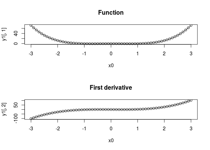
The covafillr package provides a plugin for
inline.
library(inline)The following code does local polynomial regression at the point x
based on the observations obs at the points coord. For convenience, the
plugin provides the type definitions cVector and
cMatrix to pass to the covafill constructor
and operator.
cftest <- '
  cVector x1 = as<cVector>(x);
  cMatrix coord1 = as<cMatrix>(coord);
  cVector obs1 = as<cVector>(obs);
  int p1 = as<int>(p);
  cVector h1 = as<cVector>(h);
  covafill<double> cf(coord1,obs1,h1,p1);
  return wrap(cf(x1));'
An R function can now be defined with inlined C++ code
using plugin='covafillr'.
fun <- cxxfunction(signature(x='numeric',
                             coord = 'matrix',
                             obs = 'numeric',
                             p = 'integer',
                             h = 'numeric'),
                   body = cftest,
                   plugin = 'covafillr'
) fun(c(0),matrix(x,ncol=1),y,2,1.0)## [1] -0.03907458 -0.01879995To use covafillr with TMB, include
covafill/TMB in the beginning of the cpp file.
// tmb_covafill.cpp
#include <TMB.hpp>
#include <covafill/TMB>

template<class Type>
Type objective_function<Type>::operator() ()
{
  DATA_MATRIX(coord);
  DATA_VECTOR(covObs);
  DATA_INTEGER(p);
  DATA_VECTOR(h);
  PARAMETER_VECTOR(x);
  covafill<Type> cf(coord,covObs,h,p);
  Type val = evalFill((CppAD::vector<Type>)x, cf)[0];
  return val;
}
Instead of calling the usual operator, the covafill object is
evaluated at a point with the evalFill function. This
function enables TMB to use the estimated gradient in the automatic
differentiation.
From R, the cpp file must be compiled with additional
flags as seen below.
library(TMB)
TMB::compile('tmb_covafill.cpp',CXXFLAGS = cxxFlags())
## Note: Using Makevars in /home/cmoe/.R/Makevars
## [1] 0dyn.load(dynlib("tmb_covafill"))Then TMB can be used as usual.
dat <- list(coord = matrix(x,ncol=1),
            covObs = y,
            p = 2,
            h = 1.0)

obj <- MakeADFun(data = dat,
                 parameters = list(x = c(0)),
DLL = "tmb_covafill")obj$fn(c(3.2))## [1] 94.50085obj$fn(c(0))## [1] -0.03907458obj$fn(c(-1))## [1] -0.05840993obj$gr()## outer mgc: 3.661488
## [,1]
## [1,] -3.661488library(rjags)## Loading required package: coda
## Linked to JAGS 4.0.0
## Loaded modules: basemod,bugsIf covafillr is installed with JAGS, a
module is compiled with the package. The module can be loaded in
R by the function loadJAGSModule, a wrapper
for rjags::load.module.
loadJAGSModule()## module covafillr loadedThen the function covafill is available to use in the
JAGS code
# covafill.jags
model {
  cf <- covafill(x,obsC,obs,h,2.0)
  sigma ~ dunif(0,100)
  tau <- pow(sigma, -2)
  for(i in 1:N) {
    y[i] ~ dnorm(cf[i],tau)
  }
}
fun <- function(x) x ^ 2
n <- 100
x <- runif(n,-2,2)
y <- rnorm(n,fun(x),0.5)
obsC <- seq(-3,3,len=1000)
obs <- fun(obsC) + rnorm(length(obsC),0,0.1)Then rjags can be used as usual.
jags <- jags.model('covafill.jags',
                   data = list(N = n,
                               x = matrix(x,ncol=1),
                               y = y,
                               obsC = matrix(obsC,ncol=1),
                               obs = obs,
                               h = c(1)),
                   n.chains = 1,
                   n.adapt = 100)
## Compiling model graph
## Resolving undeclared variables
## Allocating nodes
## Graph information:
## Observed stochastic nodes: 100
## Unobserved stochastic nodes: 1
## Total graph size: 2314
##
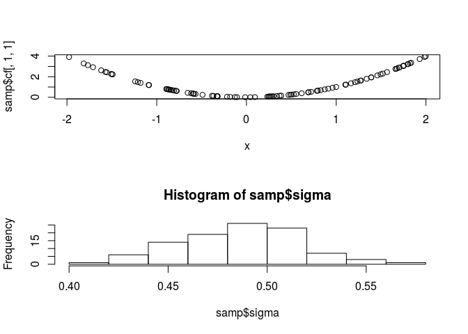
## Initializing modelsamp <- jags.samples(jags,c('sigma','cf'),n.iter = 1000, thin = 10)par(mfrow=c(2,1))
plot(x,samp$cf[,1,1])
hist(samp$sigma)