
bimets is an R package developed with the aim to ease time series analysis and to build up a framework that facilitates the definition, estimation, and simulation of simultaneous equation models.
bimets does not depend on compilers or third-party software so it can be freely downloaded and installed on Linux, MS Windows(R) and Mac OsX(R), without any further requirements.
Please consider reading the package vignette, wherein there are figures and the mathematical expressions are better formatted than in html.
If you have general questions about using bimets, or for bug reports, please use the git issue tracker or write to the maintainer.
TIME SERIES
ts[[year,period]] or ts[[start]] or
ts[[start,end]], given
start<-c(year1,period1) and
end<-c(year2,period2) and ts as a time
series.ts['Date'], or multiple
observations by using ts['StartDate/EndDate'].ts[indices].STOCK, SUM, AVE, etc.)
while reducing the time series frequency.TSEXTEND(), time series merging TSMERGE(),
time series projection TSPROJECT(), lag
TSLAG(), lag differences absolute and percentage
TSDELTA() TSDELTAP(), cumulative product
CUMPROD(), cumulative sum CUMSUM(), moving
average MOVAVG(), moving sum MOVSUM(), time
series data presentation TABIT().BIMETS2CSV() and
CSV2BIMETS().Example:
#create ts
myTS=TIMESERIES((1:100),START=c(2000,1),FREQ='D')

myTS[1:3]                         #get first three obs.
myTS[[2000,14]]                   #get year 2000 period 14
myTS[[2032,1]]                    #get year 2032 period 1 (out of range)

start <- c(2000,20)
end   <- c(2000,30)
myTS[[start]]                     #get year 2000 period 20
myTS[[start,end]]                 #get from year-period 2000-20 to 2000-30

myTS['2000-01-12']                #get Jan 12, 2000
myTS['2000-02-03/2000-03-04']     #get Feb 3 up to Mar 4

myTS[[2000,3]]     <- pi          #assign to Jan 3, 2000
myTS[[2000,42]]    <- NA          #assign to Feb 11, 2000
myTS[[2000,100]]   <- c(-1,-2,-3) #assign array starting from period 100 (i.e. extend series)

myTS[[start]]     <- NA           #assign to year-period 2000-20
myTS[[start,end]] <- 3.14         #assign from year-period 2000-20 to 2000-30
myTS[[start,end]] <- -(1:11)      #assign multiple values
                                  #from year-period 2000-20 to 2000-30

myTS['2000-01-15'] <- 42          #assign to Jan 15, 2000

#aggregation/disaggregation
myMonthlyTS <- TIMESERIES(1:100,START=c(2000,1),FREQ='M')
myYearlyTS  <- YEARLY(myMonthlyTS,'AVE')
myDailyTS   <- DAILY(myMonthlyTS,'INTERP_CENTER')

#create and manipulate time series
myTS1 <- TIMESERIES(1:100,START=c(2000,1),FREQ='M')
myTS2 <- TIMESERIES(-(1:100),START=c(2005,1),FREQ='M')

#extend time series
myExtendedTS <- TSEXTEND(myTS1,UPTO = c(2020,4),EXTMODE = 'QUADRATIC')

#merge two time series
myMergedTS <-TSMERGE(myExtendedTS,myTS2,fun = 'SUM')

#project time series
myProjectedTS <- TSPROJECT(myMergedTS,TSRANGE = c(2004,2,2006,4))

#lag time series
myLagTS <- TSLAG(myProjectedTS,2)

#percentage delta of time series
myDeltaPTS <- TSDELTAP(myLagTS,2)

#moving average of time series
myMovAveTS <- MOVAVG(myDeltaPTS,5)

#print data
TABIT(myMovAveTS,myTS1)

#     Date, Prd., myMovAveTS     , myTS1
#
# Jan 2000, 1   ,                ,  1
# Feb 2000, 2   ,                ,  2
# Mar 2000, 3   ,                ,  3
# ...
# Sep 2004, 9   ,                ,  57
# Oct 2004, 10  ,  3.849002      ,  58
# Nov 2004, 11  ,  3.776275      ,  59
# Dec 2004, 12  ,  3.706247      ,  60
# Jan 2005, 1   ,  3.638771      ,  61
# Feb 2005, 2   ,  3.573709      ,  62
# Mar 2005, 3   ,  3.171951      ,  63
# Apr 2005, 4   ,  2.444678      ,  64
# May 2005, 5   ,  1.730393      ,  65
# Jun 2005, 6   ,  1.028638      ,  66
# Jul 2005, 7   ,  0.3389831     ,  67
# Aug 2005, 8   ,  0             ,  68
# Sep 2005, 9   ,  0             ,  69
# Oct 2005, 10  ,  0             ,  70
# ...
# Mar 2008, 3   ,                ,  99
# Apr 2008, 4   ,                ,  100

#save to CSV
csvOut <- list(
  mySeries1=myTS1,
  mySeries2=myMovAveTS
)

BIMETS2CSV(csvOut, filePath='temp.csv', mergeList=TRUE, overWrite=TRUE)
More details are available in the reference manual.
MODELING:
bimets econometric modeling capabilities comprehend:
character R variable with a specific syntax. Collectively,
these keyword statements constitute a kind of a bimets
Model Description Language (i.e. MDL). The MDL syntax
allows the definition of behavioral equations, technical equations,
conditional evaluations during the simulation, and other model
properties.ESTIMATE() supports Ordinary Least Squares, Instrumental
Variables, deterministic linear restrictions on the coefficients, Almon
Polynomial Distributed Lags (i.e. PDL), autocorrelation of
the errors, structural stability analysis (Chow tests).SIMULATE() supports static, dynamic and forecast
simulations, residuals check, partial or total exogenization of
endogenous variables, constant adjustment of endogenous variables
(i.e. add-factors).TSLEAD
function in theirs equations applied to an endogenous variable;
Forward-looking models assume that economic agents have complete
knowledge of an economic system and calculate the future value of
economic variables correctly according to that knowledge. Thus,
forward-looking models are called also rational expectations models and,
in macro-econometric models, model-consistent expectations.STOCHSIMULATE() the structural disturbances are
given values that have specified stochastic properties. The error terms
of the estimated behavioral equation of the model are appropriately
perturbed. Identity equations and exogenous variables can be as well
perturbed by disturbances that have specified stochastic properties. The
model is then solved for each data set with different values of the
disturbances. Finally, mean and standard deviation are computed for each
simulated endogenous variable.MULTMATRIX() computes the matrix of both impact
and interim multipliers for a selected set of endogenous variables,
i.e. the TARGET, with respect to a selected set of
exogenous variables, i.e. the INSTRUMENT.RENORM() performs the endogenous targeting of econometric
models, which consists of solving the model while interchanging the role
of one or more endogenous variables with an equal number of exogenous
variables. The procedure determines the values for the
INSTRUMENT exogenous variables that allow achieving the
desired values for the TARGET endogenous variables, subject
to the constraints given by the equations of the model. This is an
approach to economic and monetary policy analysis.A Klein’s model example, having restrictions, error autocorrelation, and conditional evaluations, follows. For more realistic scenarios, several advanced econometric exercises on the US Federal Reserve FRB/US econometric model (e.g., dynamic simulation in a monetary policy shock, rational expectations, endogenous targeting, stochastic simulation, etc.) are available in the “US Federal Reserve quarterly model (FRB/US) in R with bimets” vignette:
# MODEL DEFINITION AND LOADING #################################################

#define the Klein model
klein1.txt <- "MODEL

COMMENT> Modified Klein Model 1 of the U.S. Economy with PDL,
COMMENT> autocorrelation on errors, restrictions, and conditional equation evaluations

COMMENT> Consumption with autocorrelation on errors
BEHAVIORAL> cn
TSRANGE 1923 1 1940 1
EQ> cn =  a1 + a2*p + a3*TSLAG(p,1) + a4*(w1+w2)
COEFF> a1 a2 a3 a4
ERROR> AUTO(2)

COMMENT> Investment with restrictions
BEHAVIORAL> i
TSRANGE 1923 1 1940 1
EQ> i = b1 + b2*p + b3*TSLAG(p,1) + b4*TSLAG(k,1)
COEFF> b1 b2 b3 b4
RESTRICT> b2 + b3 = 1

COMMENT> Demand for Labor with PDL
BEHAVIORAL> w1
TSRANGE 1923 1 1940 1
EQ> w1 = c1 + c2*(y+t-w2) + c3*TSLAG(y+t-w2,1) + c4*time
COEFF> c1 c2 c3 c4
PDL> c3 1 2

COMMENT> Gross National Product
IDENTITY> y
EQ> y = cn + i + g - t

COMMENT> Profits
IDENTITY> p
EQ> p = y - (w1+w2)

COMMENT> Capital Stock with IF switches
IDENTITY> k
EQ> k = TSLAG(k,1) + i
IF> i > 0
IDENTITY> k
EQ> k = TSLAG(k,1)
IF> i <= 0

END"

#load the model
kleinModel <- LOAD_MODEL(modelText = klein1.txt)

# Loading model: "klein1.txt"...
# Analyzing behaviorals...
# Analyzing identities...
# Optimizing...
# Loaded model "klein1.txt":
#     3 behaviorals
#     3 identities
#    12 coefficients
# ...LOAD MODEL OK

kleinModel$behaviorals$cn
# $eq
# [1] "cn=a1+a2*p+a3*TSLAG(p,1)+a4*(w1+w2)"
#
# $eqCoefficientsNames
# [1] "a1" "a2" "a3" "a4"
#
# $eqComponentsNames
# [1] "cn" "p"  "w1" "w2"
#
# $tsrange
# [1] 1925    1 1941    1
#
# $eqRegressorsNames
# [1] "1"         "p"        "TSLAG(p,1)" "(w1+w2)"
#
# $eqSimExp
# expression(cn[2,]=cn__ADDFACTOR[2,]+cn__a1+cn__a2*p[2,]+cn__a3*...
#
# ...and more

kleinModel$incidence_matrix

#    cn i w1 y p k
# cn  0 0  1 0 1 0
# i   0 0  0 0 1 0
# w1  0 0  0 1 0 0
# y   1 1  0 0 0 0
# p   0 0  1 1 0 0
# k   0 1  0 0 0 0
#define data
kleinModelData <- list(
    cn  =TIMESERIES(39.8,41.9,45,49.2,50.6,52.6,55.1,56.2,57.3,57.8,
                 55,50.9,45.6,46.5,48.7,51.3,57.7,58.7,57.5,61.6,65,69.7,
                 START=c(1920,1),FREQ=1),
    g   =TIMESERIES(4.6,6.6,6.1,5.7,6.6,6.5,6.6,7.6,7.9,8.1,9.4,10.7,
                 10.2,9.3,10,10.5,10.3,11,13,14.4,15.4,22.3,
                 START=c(1920,1),FREQ=1),
    i   =TIMESERIES(2.7,-.2,1.9,5.2,3,5.1,5.6,4.2,3,5.1,1,-3.4,-6.2,
                 -5.1,-3,-1.3,2.1,2,-1.9,1.3,3.3,4.9,
                 START=c(1920,1),FREQ=1),
    k   =TIMESERIES(182.8,182.6,184.5,189.7,192.7,197.8,203.4,207.6,
                 210.6,215.7,216.7,213.3,207.1,202,199,197.7,199.8,
                 201.8,199.9,201.2,204.5,209.4,
                 START=c(1920,1),FREQ=1),
    p   =TIMESERIES(12.7,12.4,16.9,18.4,19.4,20.1,19.6,19.8,21.1,21.7,
                 15.6,11.4,7,11.2,12.3,14,17.6,17.3,15.3,19,21.1,23.5,
                 START=c(1920,1),FREQ=1),
    w1  =TIMESERIES(28.8,25.5,29.3,34.1,33.9,35.4,37.4,37.9,39.2,41.3,
                 37.9,34.5,29,28.5,30.6,33.2,36.8,41,38.2,41.6,45,53.3,
                 START=c(1920,1),FREQ=1),
    y   =TIMESERIES(43.7,40.6,49.1,55.4,56.4,58.7,60.3,61.3,64,67,57.7,
                 50.7,41.3,45.3,48.9,53.3,61.8,65,61.2,68.4,74.1,85.3,
                 START=c(1920,1),FREQ=1),
    t   =TIMESERIES(3.4,7.7,3.9,4.7,3.8,5.5,7,6.7,4.2,4,7.7,7.5,8.3,5.4,
                 6.8,7.2,8.3,6.7,7.4,8.9,9.6,11.6,
                 START=c(1920,1),FREQ=1),
    time=TIMESERIES(NA,-10,-9,-8,-7,-6,-5,-4,-3,-2,-1,0,
                 1,2,3,4,5,6,7,8,9,10,
                 START=c(1920,1),FREQ=1),
    w2  =TIMESERIES(2.2,2.7,2.9,2.9,3.1,3.2,3.3,3.6,3.7,4,4.2,4.8,
                 5.3,5.6,6,6.1,7.4,6.7,7.7,7.8,8,8.5,
                 START=c(1920,1),FREQ=1)
    );

kleinModel <- LOAD_MODEL_DATA(kleinModel,kleinModelData)
# Load model data "kleinModelData" into model "klein1.txt"...
# ...LOAD MODEL DATA OK


# MODEL ESTIMATION #############################################################

kleinModel <- ESTIMATE(kleinModel)
#.CHECK_MODEL_DATA(): warning, there are undefined values in time series "time".
#
#Estimate the Model klein1.txt:
#the number of behavioral equations to be estimated is 3.
#The total number of coefficients is 13.
#
#_________________________________________
#
#BEHAVIORAL EQUATION: cn
#Estimation Technique: OLS
#Autoregression of Order  2  (Cochrane-Orcutt procedure)
#
#Convergence was reached in  6  /  20  iterations.
#
#
#cn                  =   14.82685
#                        T-stat. 7.608453    ***
#
#                    +   0.2589094   p
#                        T-stat. 2.959808    *
#
#                    +   0.01423821  TSLAG(p,1)
#                        T-stat. 0.1735191
#
#                    +   0.8390274   (w1+w2)
#                        T-stat. 14.67959    ***
#
#ERROR STRUCTURE:  AUTO(2)
#
#AUTOREGRESSIVE PARAMETERS:
#Rho             Std. Error      T-stat.
# 0.2542111       0.2589487       0.9817045
#-0.05250591      0.2593578      -0.2024458
#
#
#STATs:
#R-Squared                      : 0.9826778
#Adjusted R-Squared             : 0.9754602
#Durbin-Watson Statistic        : 2.256004
#Sum of squares of residuals    : 8.071633
#Standard Error of Regression   : 0.8201439
#Log of the Likelihood Function : -18.32275
#F-statistic                    : 136.1502
#F-probability                  : 3.873514e-10
#Akaike's IC                    : 50.6455
#Schwarz's IC                   : 56.8781
#Mean of Dependent Variable     : 54.29444
#Number of Observations         : 18
#Number of Degrees of Freedom   : 12
#Current Sample (year-period)   : 1923-1 / 1940-1
#
#
#Signif. codes:   *** 0.001  ** 0.01  * 0.05
#
#
# ...similar output for all the regressions.


# MODEL SIMULATION #############################################################

#simulate GNP in 1925-1930
kleinModel <- SIMULATE(kleinModel,
                      TSRANGE=c(1925,1,1930,1),
                      simIterLimit = 100)

# Simulation:    100.00%
# ...SIMULATE OK

#print simulated GNP
TABIT(kleinModel$simulation$y)
#
#      Date, Prd., kleinModel$simulation$y
#
#      1925, 1   ,  58.24584
#      1926, 1   ,  44.56501
#      1927, 1   ,  28.2727
#      1928, 1   ,  27.10598
#      1929, 1   ,  37.57604
#      1930, 1   ,  37.44899

#save simulated time series to csv
BIMETS2CSV(
  kleinModel$simulation[kleinModel$vendog],
  filePath='temp.csv',
  mergeList=TRUE,
  overWrite=TRUE)

# MODEL STOCHASTIC FORECAST ####################################################

#we want to perform a stochastic forecast of the GNP up to 1944
#we will add normal disturbances to endogenous Consumption 'cn'
#in 1942 by using its regression standard error
#we will add uniform disturbances to exogenous Government Expenditure 'g'
#in whole TSRANGE
myStochStructure <- list(
  cn=list(
        TSRANGE=c(1942,1,1942,1),
        TYPE='NORM',
        PARS=c(0,kleinModel$behaviorals$cn$statistics$StandardErrorRegression)
        ),
  g=list(
        TSRANGE=TRUE,
        TYPE='UNIF',
        PARS=c(-1,1)
        )
  )

#we need to extend exogenous variables up to 1944
kleinModel$modelData <- within(kleinModel$modelData,{
    w2    = TSEXTEND(w2,  UPTO=c(1944,1),EXTMODE='CONSTANT')
    t     = TSEXTEND(t,   UPTO=c(1944,1),EXTMODE='LINEAR')
    g     = TSEXTEND(g,   UPTO=c(1944,1),EXTMODE='CONSTANT')
    k     = TSEXTEND(k,   UPTO=c(1944,1),EXTMODE='LINEAR')
    time  = TSEXTEND(time,UPTO=c(1944,1),EXTMODE='LINEAR')
  })

#stochastic model forecast
kleinModel <- STOCHSIMULATE(kleinModel
                      ,simType='FORECAST'
                      ,TSRANGE=c(1941,1,1944,1)
                      ,StochStructure=myStochStructure
                      ,StochSeed=123
                      )

#print mean and standard deviation of forecasted GNP
with(kleinModel$stochastic_simulation,TABIT(y$mean, y$sd))

#      Date, Prd., y$mean         , y$sd
#
#      1941, 1   ,  125.5045      ,  4.250935
#      1942, 1   ,  173.2946      ,  9.2632
#      1943, 1   ,  185.9602      ,  11.87774
# 1944, 1 , 141.0807 , 11.6973 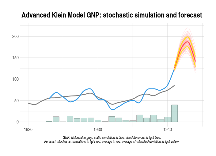
# MODEL MULTIPLIERS  ###########################################################

#get multiplier matrix in 1941
kleinModel <- MULTMATRIX(kleinModel,
                        TSRANGE=c(1941,1,1941,1),
                        INSTRUMENT=c('w2','g'),
                        TARGET=c('cn','y'),
                        simIterLimit = 100)

# Multiplier Matrix:    100.00%
# ...MULTMATRIX OK

kleinModel$MultiplierMatrix
#           w2_1      g_1
#cn_1  0.2338194 3.753277
#y_1  -0.2002040 7.444930


# MODEL ENDOGENOUS TARGETING ###################################################

#we want an arbitrary value on Consumption of 66 in 1940 and 78 in 1941
#we want an arbitrary value on GNP of 77 in 1940 and 98 in 1941
kleinTargets  <-  list(
                    cn = TIMESERIES(66,78,START=c(1940,1),FREQ=1),
                    y  = TIMESERIES(77,98,START=c(1940,1),FREQ=1)
                    )
#Then, we can perform the model endogenous targeting
#by using Government Wage Bill 'w2'
#and Government Expenditure 'g' as
#INSTRUMENT in the years 1940 and 1941:
kleinModel <- RENORM(kleinModel
                   ,simConvergence=1e-5
                   ,INSTRUMENT = c('w2','g')
                   ,TARGET = kleinTargets
                   ,TSRANGE = c(1940,1,1941,1)
                   ,simIterLimit = 100
                    )

# Convergence reached in 3 iterations.
# ...RENORM OK

#The calculated values of exogenous INSTRUMENT
#that allow achieving the desired endogenous TARGET values
#are stored into the model:

with(kleinModel,TABIT(modelData$w2,
                      renorm$INSTRUMENT$w2,
                      modelData$g,
                      renorm$INSTRUMENT$g))

#       Date, Prd., modelData$w2,  renorm$w2, modelData$g, renorm$g
#
#       ...
#
#      1938, 1   ,  7.7           ,                ,  13            ,
#      1939, 1   ,  7.8           ,                ,  14.4          ,
#      1940, 1   ,  8             ,  5.577777      ,  15.4          ,  14.14058
#      1941, 1   ,  8.5           ,  5.354341      ,  22.3          ,  17.80586

#So, if we want to achieve on "cn" (Consumption) an arbitrary simulated value of 66 in 1940
#and 78 in 1941, and if we want to achieve on "y" (GNP) an arbitrary simulated value of 77
#in 1940 and 98 in 1941, we need to change exogenous "w2" (Wage Bill of the Government
#Sector) from 8 to 5.58 in 1940 and from 8.5 to 5.35 in 1941, and we need to change exogenous
#"g"(Government Expenditure) from 15.4 to 14.14 in 1940 and from 22.3 to 17.81 in 1941.

#Let's verify:

#create a new model
kleinRenorm <- kleinModel

#update the required INSTRUMENT
kleinRenorm$modelData <- kleinRenorm$renorm$modelData

#simulate the new model
kleinRenorm <- SIMULATE(kleinRenorm
                  ,TSRANGE=c(1940,1,1941,1)
                  ,simConvergence=1e-4
                  ,simIterLimit=100
                  )
#Simulation:    100.00%
#...SIMULATE OK

#verify TARGETs are achieved
with(kleinRenorm$simulation,
    TABIT(cn,y)
    )

#      Date, Prd., cn             , y
#
#      1940, 1   ,  65.99977      ,  76.9996
#      1941, 1   ,  77.99931      ,  97.99879

# MODEL OPTIMAL CONTROL ########################################################

#reset time series data in model
kleinModel <- LOAD_MODEL_DATA(kleinModel
                              ,kleinModelData
                              ,quietly = TRUE)

#we want to maximize the non-linear objective function:
#f()=(y-110)+(cn-90)*ABS(cn-90)-(g-20)^0.5
#in 1942 by using INSTRUMENT cn in range (-5,5)
#(cn is endogenous so we use the add-factor)
#and g in range (15,25)
#we will also impose the following non-linear restriction:
#g+(cn^2)/2<27 & g+cn>17

#we need to extend exogenous variables up to 1942
kleinModel$modelData <- within(kleinModel$modelData,{
    w2    = TSEXTEND(w2,   UPTO = c(1942,1), EXTMODE = 'CONSTANT')
    t     = TSEXTEND(t,    UPTO = c(1942,1), EXTMODE = 'LINEAR')
    g     = TSEXTEND(g,    UPTO = c(1942,1), EXTMODE = 'CONSTANT')
    k     = TSEXTEND(k,    UPTO = c(1942,1), EXTMODE = 'LINEAR')
    time  = TSEXTEND(time, UPTO = c(1942,1), EXTMODE = 'LINEAR')
})

#define INSTRUMENT and boundaries
myOptimizeBounds <- list(
    cn = list( TSRANGE = TRUE
            ,BOUNDS = c(-5,5)),
     g = list( TSRANGE = TRUE
            ,BOUNDS = c(15,25))
)

#define restrictions
myOptimizeRestrictions <- list(
    myRes1=list(
         TSRANGE = TRUE
        ,INEQUALITY = 'g+(cn^2)/2<27 & g+cn>17')
)

#define objective function
myOptimizeFunctions <- list(
    myFun1 = list(
         TSRANGE = TRUE
        ,FUNCTION = '(y-110)+(cn-90)*ABS(cn-90)-(g-20)^0.5')
)

#Monte-Carlo optimization by using 10.000 stochastic realizations
#and 1E-7 convergence criterion
kleinModel <- OPTIMIZE(kleinModel
                        ,simType = 'FORECAST'
                        ,TSRANGE=c(1942,1,1942,1)
                        ,simConvergence= 1E-7
                        ,simIterLimit  = 100
                        ,StochReplica  = 10000
                        ,StochSeed = 123
                        ,OptimizeBounds = myOptimizeBounds
                        ,OptimizeRestrictions = myOptimizeRestrictions
                        ,OptimizeFunctions = myOptimizeFunctions
                        ,quietly = TRUE)

#print local maximum
kleinModel$optimize$optFunMax
#[1] 210.577

#print INSTRUMENT that allow local maximum to be achieved
kleinModel$optimize$INSTRUMENT
#$cn
#Time Series:
#Start = 1942
#End = 1942
#Frequency = 1
#[1] 2.032203
#
#$g
#Time Series:
#Start = 1942
#End = 1942
#Frequency = 1
#[1] 24.89773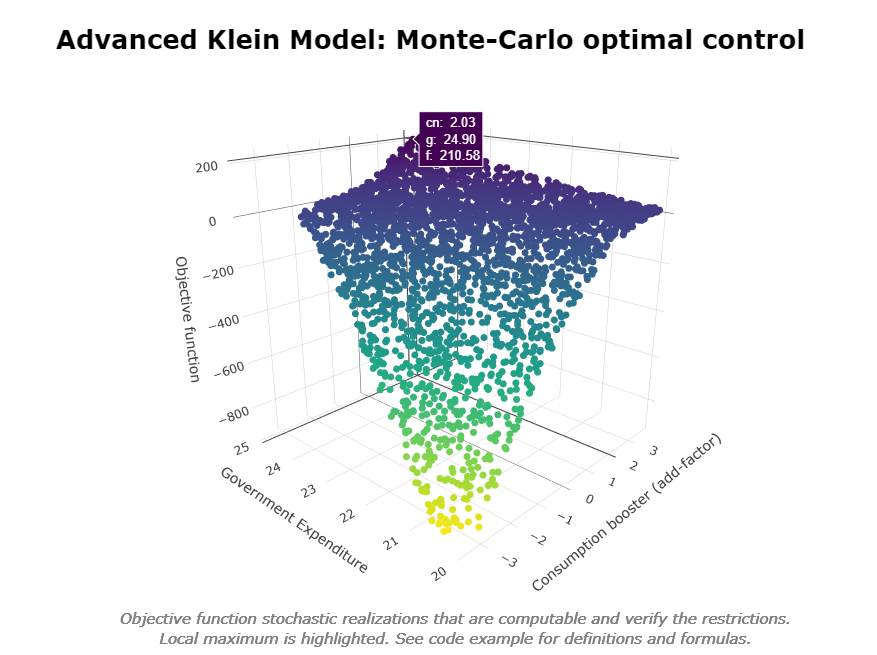
# RATIONAL EXPECTATIONS ########################################################

# EXAMPLE OF FORWARD-LOOKING KLEIN-LIKE MODEL
# HAVING RATIONAL EXPECTATION ON INVESTMENTS

#define model
kleinLeadModelDefinition<-
"MODEL
COMMENT> Klein Model 1 of the U.S. Economy

COMMENT> Consumption
BEHAVIORAL> cn
TSRANGE 1921 1 1941 1
EQ> cn =  a1 + a2*p + a3*TSLAG(p,1) + a4*(w1+w2)
COEFF> a1 a2 a3 a4

COMMENT> Investment with TSLEAD
IDENTITY> i
EQ> i = (MOVAVG(i,2)+TSLEAD(i))/2

COMMENT> Demand for Labor
BEHAVIORAL> w1
TSRANGE 1921 1 1941 1
EQ> w1 = c1 + c2*(y+t-w2) + c3*TSLAG(y+t-w2,1) + c4*time
COEFF> c1 c2 c3 c4

COMMENT> Gross National Product
IDENTITY> y
EQ> y = cn + i + g - t

COMMENT> Profits
IDENTITY> p
EQ> p = y - (w1+w2)

COMMENT> Capital Stock
IDENTITY> k
EQ> k = TSLAG(k,1) + i

END"

#define model data
kleinLeadModelData<-list(
  cn
  =TIMESERIES(39.8,41.9,45,49.2,50.6,52.6,55.1,56.2,57.3,57.8,55,50.9,
              45.6,46.5,48.7,51.3,57.7,58.7,57.5,61.6,65,69.7,
              START=c(1920,1),FREQ=1),
  g
  =TIMESERIES(4.6,6.6,6.1,5.7,6.6,6.5,6.6,7.6,7.9,8.1,9.4,10.7,10.2,9.3,10,
              10.5,10.3,11,13,14.4,15.4,22.3,
              START=c(1920,1),FREQ=1),
  i
  =TIMESERIES(2.7,-.2,1.9,5.2,3,5.1,5.6,4.2,3,5.1,1,-3.4,-6.2,-5.1,-3,-1.3,
              2.1,2,-1.9,1.3,3.3,4.9,
              START=c(1920,1),FREQ=1),
  k
  =TIMESERIES(182.8,182.6,184.5,189.7,192.7,197.8,203.4,207.6,210.6,215.7,
              216.7,213.3,207.1,202,199,197.7,199.8,201.8,199.9,
              201.2,204.5,209.4,
              START=c(1920,1),FREQ=1),
  p
  =TIMESERIES(12.7,12.4,16.9,18.4,19.4,20.1,19.6,19.8,21.1,21.7,15.6,11.4,
              7,11.2,12.3,14,17.6,17.3,15.3,19,21.1,23.5,
              START=c(1920,1),FREQ=1),
  w1
  =TIMESERIES(28.8,25.5,29.3,34.1,33.9,35.4,37.4,37.9,39.2,41.3,37.9,34.5,
              29,28.5,30.6,33.2,36.8,41,38.2,41.6,45,53.3,
              START=c(1920,1),FREQ=1),
  y
  =TIMESERIES(43.7,40.6,49.1,55.4,56.4,58.7,60.3,61.3,64,67,57.7,50.7,41.3,
              45.3,48.9,53.3,61.8,65,61.2,68.4,74.1,85.3,
              START=c(1920,1),FREQ=1),
  t
  =TIMESERIES(3.4,7.7,3.9,4.7,3.8,5.5,7,6.7,4.2,4,7.7,7.5,8.3,5.4,6.8,7.2,
              8.3,6.7,7.4,8.9,9.6,11.6,
              START=c(1920,1),FREQ=1),
  time
  =TIMESERIES(NA,-10,-9,-8,-7,-6,-5,-4,-3,-2,-1,0,1,2,3,4,5,6,7,8,9,10,
              START=c(1920,1),FREQ=1),
  w2
  =TIMESERIES(2.2,2.7,2.9,2.9,3.1,3.2,3.3,3.6,3.7,4,4.2,4.8,5.3,5.6,6,6.1,
              7.4,6.7,7.7,7.8,8,8.5,
              START=c(1920,1),FREQ=1)
)

#load model and model data
kleinLeadModel<-LOAD_MODEL(modelText=kleinLeadModelDefinition)
kleinLeadModel<-LOAD_MODEL_DATA(kleinLeadModel,kleinLeadModelData)

#estimate model
kleinLeadModel<-ESTIMATE(kleinLeadModel, quietly = TRUE)

#set expected value of 2 for Investment in 1931
#(note that simulation TSRANGE spans up to 1930)
kleinLeadModel$modelData$i[[1931,1]]<-2

#simulate model
kleinLeadModel<-SIMULATE(kleinLeadModel
                  ,TSRANGE=c(1924,1,1930,1))

#print simulated investments
TABIT(kleinLeadModel$simulation$i)

#Date, Prd., kleinLeadModel$simulation$i
#
#      1924, 1   ,  3.594946
#      1925, 1   ,  2.792062
#      1926, 1   ,  2.390277
#      1927, 1   ,  2.189125
#      1928, 1   ,  2.08838
#      1929, 1   ,  2.037915
#      1930, 1   ,  2.012644
MODEL DESCRIPTION LANGUAGE SYNTAX
The mathematical expression available for use in model equations can include the standard arithmetic operators, parentheses and the following MDL functions:
TSLAG(ts,i): lag the ts time series by i-periods;TSLEAD(ts,i): lead the ts time series by
i-periods;TSDELTA(ts,i): i-periods difference of the ts time
series;TSDELTAP(ts,i): i-periods percentage difference of the
ts time series;TSDELTALOG(ts,i): i-periods logarithmic difference of
the ts time series;MOVAVG(ts,i): i-periods moving average of the ts time
series;MOVSUM(ts,i): i-periods moving sum of the ts time
series;LOG(ts): log of the ts time series;EXP(ts): exponential of the ts time series;ABS(ts): absolute values of the ts time series.Transformations of the dependent variable are allowed in
EQ> definition, e.g. TSDELTA(cn)=...,
EXP(i)=..., TSDELTALOG(y)=..., etc.
More details are available in the reference manual.
COMPUTATIONAL DETAILS
The iterative simulation procedure is the most time-consuming operation of the bimets package. For small models, this operation is quite immediate; on the other hand, the simulation of models that count hundreds of equations could last for minutes, especially if the requested operation involves a parallel simulation having hundreds of realizations per equation. This could be the case for the endogenous targeting, the stochastic simulation and the optimal control. In these cases, a Newton-Raphson algorithm can speed up the execution.
The SIMULATE code has been optimized in order to
minimize the execution time in these cases. In terms of computational
efficiency, the procedure takes advantage of the fact that multiple
datasets are bound together in matrices, therefore in order to achieve a
global convergence, the iterative simulation algorithm is executed once
for all perturbed datasets. This solution can be viewed as a sort of a
SIMD (i.e. Single Instruction Multiple Data) parallel simulation: the
SIMULATE algorithm transforms time series into matrices and
consequently can easily bind multiple datasets by column. At the same
time, the single run ensures a fast code execution, while each column in
the output matrices represents a stochastic or perturbed
realization.
The above approach is even faster if R has been compiled and linked to optimized multi-threaded numerical libraries, e.g. Intel(R) MKL, OpenBlas, Microsoft(R) R Open, etc.
Finally, model equations are pre-fetched into sorted R expressions,
and an optimized R environment is defined and reserved to the
SIMULATE algorithm; this approach removes the overhead
usually caused by expression parsing and by the R looking
for variables inside nested environments.
bimets estimation and simulation results have been compared to the output results of leading commercial econometric software by using several large and complex models.
The models used in the comparison have more than:
In these models, we can find equations with restricted coefficients, polynomial distributed lags, error autocorrelation, and conditional evaluation of technical identities; all models have been simulated in static, dynamic, and forecast mode, with exogenization and constant adjustments of endogenous variables, through the use of bimets capabilities.
In the +800 endogenous simulated time series over the +20 simulated
periods (i.e. more than 16.000 simulated observations), the average
percentage difference between bimets and leading
commercial software results has a magnitude of 10E-7 %. The
difference between results calculated by using different commercial
software has the same average magnitude.
Several advanced econometric exercises on the US Federal Reserve FRB/US econometric model (e.g., dynamic simulation in a monetary policy shock, rational expectations, endogenous targeting, stochastic simulation, etc.) are available in the “US Federal Reserve quarterly model (FRB/US) in R with bimets” vignette.
The package can be installed and loaded in R with the following commands:
install.packages("bimets")
library(bimets)We welcome contributions to the bimets package. In the case, please use the git issue tracker or write to the maintainer.
The bimets package is licensed under the GPL-3.
Disclaimer: The views and opinions expressed in these pages are those of the authors and do not necessarily reflect the official policy or position of the Bank of Italy. Examples of analysis performed within these pages are only examples. They should not be utilized in real-world analytic products as they are based only on very limited and dated open source information. Assumptions made within the analysis are not reflective of the position of the Bank of Italy.