bayesboot:
Easy Bayesian Bootstrap in RThe bayesboot package implements a function
bayesboot that performs the Bayesian bootstrap introduced
by Rubin (1981). The implementation can both handle summary statistics
that works on a weighted version of the data or that works on a
resampled data set.
bayesboot is available on CRAN and can be installed in
the usual way:
install.packages("bayesboot")Here is a Bayesian bootstrap analysis of the mean height of the last ten American presidents:
# Heights of the last ten American presidents in cm (Kennedy to Obama).
heights <- c(183, 192, 182, 183, 177, 185, 188, 188, 182, 185)
library(bayesboot)
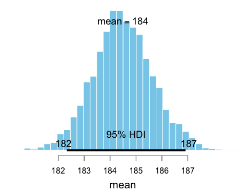
b1 <- bayesboot(heights, mean)The resulting posterior distribution in b1 can now be
plotted and summaryized:
summary(b1)
## Bayesian bootstrap
##
## Number of posterior draws: 4000
##
## Summary of the posterior (with 95% Highest Density Intervals):
##  statistic     mean       sd  hdi.low hdi.high
##         V1 184.4979 1.154456 182.3328  186.909
##
## Quantiles:
##  statistic    q2.5%    q25%   median     q75%   q97.5%
##         V1 182.2621 183.742 184.4664 185.2378 186.8737
##
## Call:
##  bayesboot(data = heights, statistic = mean)
plot(b1)
While it is possible to use a summary statistic that works on a
resample of the original data, it is more efficient if it’s possible to
use a summary statistic that works on a reweighting of the
original dataset. Instead of using mean above it would be
better to use weighted.mean like this:
b2 <- bayesboot(heights, weighted.mean, use.weights = TRUE)The result of a call to bayesboot will always result in
a data.frame with one column per dimension of the summary
statistic. If the summary statistic does not return a named vector the
columns will be called V1, V2, etc. The result
of a bayesboot call can be further inspected and post
processed. For example:
# Given the model and the data, this is the probability that the mean
# heights of American presidents is above the mean heights of
# American males as given by www.cdc.gov/nchs/data/series/sr_11/sr11_252.pdf
mean(c(b2[,1] > 175.9, TRUE, FALSE))
## [1] 0.9997501If we want to compare the means of two groups, we will have to call
bayesboot twice with each dataset and then use the
resulting samples to calculate the posterior difference. For example,
let’s say we have the heights of the opponents that lost to the
presidents in height the first time those presidents were
elected. Now we are interested in comparing the mean height of American
presidents with the mean height of presidential candidates that
lost.
# The heights of oponents of American presidents (first time they were elected).
# From Richard Nixon to John McCain
heights_opponents <- c(182, 180, 180, 183, 177, 173, 188, 185, 175)

# Running the Bayesian bootstrap for both datasets
b_presidents <- bayesboot(heights, weighted.mean, use.weights = TRUE)
b_opponents  <- bayesboot(heights_opponents, weighted.mean, use.weights = TRUE)

# Calculating the posterior difference
# (here converting back to a bayesboot object for pretty plotting)
b_diff <- as.bayesboot(b_presidents - b_opponents)
plot(b_diff)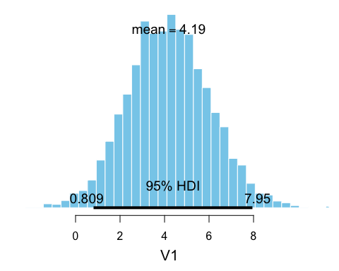
So there is some evidence that loosing opponents could be shorter. (Though, I must add that it is quite unclear what the purpose really is with analyzing the heights of presidents and opponents…)
A slightly more complicated example, where we do Bayesian bootstrap
analysis of LOESS regression applied to the cars dataset on
the speed of cars and the resulting distance it takes to stop. The
loess function returns, among other things, a vector of
fitted y values, one value for each x
value in the data. These y values define the smoothed LOESS
line and is what you would usually plot after having fitted a LOESS. Now
we want to use the Bayesian bootstrap to gauge the uncertainty in the
LOESS line. As the loess function accepts weighted data,
we’ll simply create a function that takes the data with weights and
returns the fitted y values. We’ll then plug that
function into bayesboot:
boot_fn <- function(cars, weights) {
  loess(dist ~ speed, cars, weights = weights)$fitted
}

bb_loess <- bayesboot(cars, boot_fn, use.weights = TRUE)
To plot this takes a couple of lines more:
# Plotting the data
plot(cars$speed, cars$dist, pch = 20, col = "tomato4", xlab = "Car speed in mph",
     ylab = "Stopping distance in ft", main = "Speed and Stopping distances of Cars")

# Plotting a scatter of Bootstrapped LOESS lines to represent the uncertainty.
for(i in sample(nrow(bb_loess), 20)) {
  lines(cars$speed, bb_loess[i,], col = "gray")
}
# Finally plotting the posterior mean LOESS line
lines(cars$speed, colMeans(bb_loess, na.rm = TRUE), type ="l",
      col = "tomato", lwd = 4)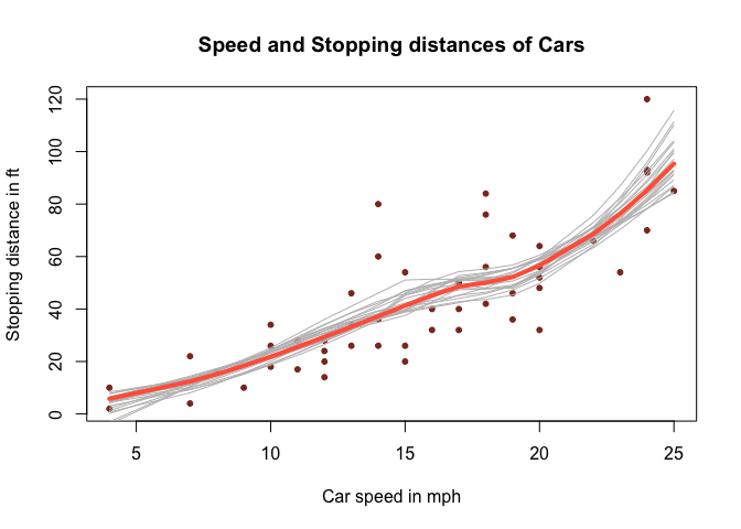
For more information on the Bayesian bootstrap see Rubin’s (1981)
original paper and my blog post The
Non-parametric Bootstrap as a Bayesian Model. The implementation of
bayesboot is similar to the function outlined in the blog
post Easy
Bayesian Bootstrap in R, but the interface is slightly
different.
Rubin, D. B. (1981). The Bayesian bootstrap. The annals of statistics, 9(1), 130–134. link to paper