![]()
The goal of {SSVS} is to provide functions for performing stochastic search variable selection (SSVS) for binary and continuous outcomes and visualizing the results. SSVS is a Bayesian variable selection method used to estimate the probability that individual predictors should be included in a regression model. Using MCMC estimation, the method samples thousands of regression models in order to characterize the model uncertainty regarding both the predictor set and the regression parameters.
You can install the development version of {SSVS} from GitHub with:
# install.packages("remotes")
remotes::install_github("sabainter/SSVS")Consider a simple example using SSVS on the mtcars
dataset to predict quarter mile times. We first specify our response
variable (“qsec”), then choose our predictors and run the
ssvs() function.
library(SSVS)
outcome <- 'qsec'
predictors <- c('cyl', 'disp', 'hp', 'drat', 'wt',
 'vs', 'am', 'gear', 'carb','mpg')

results <- ssvs(data = mtcars, x = predictors, y = outcome, progress = FALSE)
The results can be summarized and printed using the
summary() function. This will display the MIP for each
predictor, the average coefficients including and excluding zeros, and
credible intervals for each coefficient.
summary_results <- summary(results, interval = 0.9, ordered = TRUE)| Variable | MIP | Avg Beta | Avg Nonzero Beta | Lower CI (90%) | Upper CI (90%) |
|---|---|---|---|---|---|
| wt | 0.8433 | 1.0433 | 1.2372 | 0.0000 | 1.9513 |
| vs | 0.7512 | 0.6399 | 0.8519 | 0.0000 | 1.1982 |
| hp | 0.5413 | -0.4995 | -0.9228 | -1.3349 | 0.0000 |
| cyl | 0.4551 | -0.5173 | -1.1367 | -1.7670 | 0.0005 |
| am | 0.4240 | -0.3107 | -0.7328 | -1.0805 | 0.0000 |
| disp | 0.4130 | -0.4553 | -1.1023 | -1.8170 | 0.0012 |
| carb | 0.3938 | -0.2890 | -0.7338 | -1.0068 | 0.0000 |
| gear | 0.2013 | -0.0918 | -0.4560 | -0.5464 | 0.0002 |
| mpg | 0.1584 | 0.0563 | 0.3557 | -0.0001 | 0.4160 |
| drat | 0.1003 | -0.0180 | -0.1794 | -0.0008 | 0.0000 |
The MIPs for each predictor can then be visualized using the
plot() function.
plot(results)
In the example above, the response variable was a continuous
variable. The same workflow can be used for binary variables by
specifying continuous = FALSE to the ssvs()
function.
As an example, let’s create a binary variable:
library(AER)
#> Warning: package 'AER' was built under R version 4.3.3
data(Affairs)
Affairs$hadaffair[Affairs$affairs > 0] <- 1
Affairs$hadaffair[Affairs$affairs == 0] <- 0
Then define the outcome and predictors.
outcome <- "hadaffair"
predictors <- c("gender", "age", "yearsmarried", "children", "religiousness", "education", "occupation", "rating")
And finally run the model:
results <- ssvs(data = Affairs, x = predictors, y = outcome, continuous = FALSE, progress = FALSE)Now the results can be summarized or visualized in the same manner.
summary_results <- summary(results, interval = 0.9, ordered = TRUE)| Variable | MIP | Avg Beta | Avg Nonzero Beta | Lower CI (90%) | Upper CI (90%) |
|---|---|---|---|---|---|
| rating | 1.0000 | -0.5552 | -0.5552 | -0.7106 | -0.3917 |
| religiousness | 0.4247 | -0.1422 | -0.3348 | -0.4070 | 0.0000 |
| yearsmarried | 0.1035 | 0.0321 | 0.3099 | 0.0000 | 0.1024 |
| children | 0.0751 | 0.0204 | 0.2714 | 0.0000 | 0.0000 |
| age | 0.0111 | -0.0024 | -0.2146 | 0.0000 | 0.0000 |
| gender | 0.0093 | 0.0010 | 0.1067 | 0.0000 | 0.0000 |
| occupation | 0.0064 | 0.0008 | 0.1176 | 0.0000 | 0.0000 |
| education | 0.0050 | 0.0005 | 0.1066 | 0.0000 | 0.0000 |
plot(results)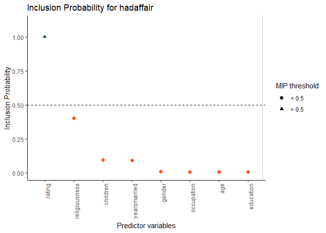
First, we will use the mice() function from the {mice}
package to perform multiple imputation.
library(mice)
#>
#> Attaching package: 'mice'
#> The following object is masked from 'package:stats':
#>
#>     filter
#> The following objects are masked from 'package:base':
#>
#>     cbind, rbind

# Load the mtcars dataset
data <- mtcars

# Introduce random missingness in 10% of the data
set.seed(123)
n <- nrow(data) * ncol(data)
missing_indices <- sample(n, size = 0.1 * n, replace = FALSE)

# Convert missing indices to row-column positions
rows <- (missing_indices - 1) %% nrow(data) + 1
cols <- (missing_indices - 1) %/% nrow(data) + 1

# Assign NA to the identified positions
for (i in seq_along(rows)) {
  data[rows[i], cols[i]] <- NA
}

# Perform multiple imputation using mice
imputed_data <- mice(data, m = 5, maxit = 50, seed = 123)

# Display the results of the imputation
summary(imputed_data)

# Extract and show the first completed dataset
imputed_mtcars <- complete(imputed_data, "long")
head(imputed_mtcars)
We will use this multiply imputed data set for SSVS, using the
ssvs_mi() function.
outcome <- 'qsec'
predictors <- c('cyl', 'disp', 'hp', 'drat', 'wt', 'vs', 'am', 'gear', 'carb','mpg')
imputation <- '.imp'
results <- ssvs_mi(data = imputed_mtcars, y = outcome, x = predictors, imp = imputation)
The results of SSVS with MI can be summarized with the
summary() and plot() functions. This will
summarize across imputations for each predictor: the average
MIP and the mean, minimum, maximum, and average nonzero beta
coefficients.
You can launch an interactive (shiny) web application that lets you
run SSVS analyses without programming. Simply install this package and
run SSVS::launch() in an R console.