

The NIMAA package [@nimaa] provides a comprehensive set of methods for performing nominal data mining.
It employs bipartite networks to demonstrate how two nominal variables are linked, and then places them in the incidence matrix to proceed with network analysis. NIMAA aids in characterizing the pattern of missing values in a dataset, locating large submatrices with non-missing values, and predicting edges within nominal variable labels. Then, given a submatrix, two unipartite networks are constructed using various network projection methods. NIMAA provides a variety of choices for clustering projected networks and selecting the best one. The best clustering results can also be used as a benchmark for imputation analysis in weighted bipartite networks.
You can install the released version of NIMAA from CRAN with:
install.packages("NIMAA")And the development version from GitHub with:
# install.packages("devtools")
devtools::install_github("jafarilab/NIMAA")library(NIMAA)
## load the beatAML data
beatAML_data <- NIMAA::beatAML
# plot the original data
beatAML_incidence_matrix <- plotIncMatrix(
x = beatAML_data, # original data with 3 columns
index_nominal = c(2,1), # the first two columns are nominal data
index_numeric = 3, # the third column is numeric data
print_skim = FALSE, # if you want to check the skim output, set this as TRUE
plot_weight = TRUE, # when plotting the weighted incidence matrix
verbose = FALSE # NOT save the figures to local folder
)
#>
#> Na/missing values Proportion: 0.2603
plotBipartite(inc_mat = beatAML_incidence_matrix, vertex.label.display = T)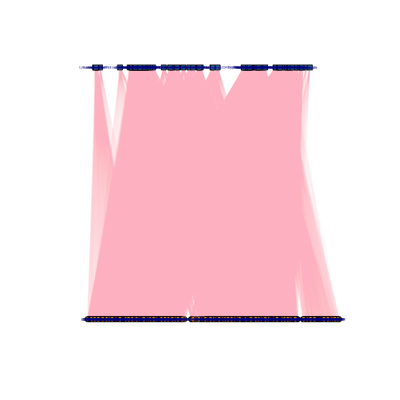
#> IGRAPH 7cf38ef UNWB 650 47636 --
#> + attr: name (v/c), type (v/l), shape (v/c), color (v/c), weight (e/n)
#> + edges from 7cf38ef (vertex names):
#>  [1] Alisertib (MLN8237)      --11-00261 Barasertib (AZD1152-HQPA)--11-00261
#>  [3] Bortezomib (Velcade)     --11-00261 Canertinib (CI-1033)     --11-00261
#>  [5] Crenolanib               --11-00261 CYT387                   --11-00261
#>  [7] Dasatinib                --11-00261 Doramapimod (BIRB 796)   --11-00261
#>  [9] Dovitinib (CHIR-258)     --11-00261 Erlotinib                --11-00261
#> [11] Flavopiridol             --11-00261 GDC-0941                 --11-00261
#> [13] Gefitinib                --11-00261 Go6976                   --11-00261
#> [15] GW-2580                  --11-00261 Idelalisib               --11-00261
#> + ... omitted several edgesThe extractSubMatrix() function extracts the submatrices
that have non-missing values or have a certain percentage of missing
values inside (not for elements-max matrix), depending on the argument’s
input. The package vignette and help manual contain more details.
sub_matrices <- extractSubMatrix(
  x = beatAML_incidence_matrix,
  shape = c("Square", "Rectangular_element_max"), # the selected shapes of submatrices
  row.vars = "patient_id",
  col.vars = "inhibitor",
  plot_weight = TRUE,
  print_skim = FALSE
  )
#> binmatnest2.temperature
#>                20.12539
#> Size of Square:   96 rows x  96 columns
#> Size of Rectangular_element_max:      87 rows x  140 columns

The findCluster() function implements seven widely used
network clustering algorithms, with the option of preprocessing the
input incidence matrix following the projecting of the bipartite network
into unipartite networks. Also, internal and external measurements can
be used to compare clustering algorithms. Details can be found in the
package vignette and help manual.
cls <- findCluster(
  sub_matrices$Rectangular_element_max,
  part = 1,
  method = "all", # all available clustering methods
  normalization = TRUE, # normalize the input matrix
  rm_weak_edges = TRUE, # remove the weak edges in the network
  rm_method = 'delete', # delete the weak edges instead of lowering their weights to 0.
  threshold = 'median', # Use median of edges' weights as threshold
  set_remaining_to_1 = TRUE, # set the weights of remaining edges to 1
  )
#> Warning in findCluster(sub_matrices$Rectangular_element_max, part = 1, method =
#> "all", : cluster_spinglass cannot work with unconnected graph
#>
#>
#> |             |  walktrap|   louvain|   infomap| label_prop| leading_eigen| fast_greedy|
#> |:------------|---------:|---------:|---------:|----------:|-------------:|-----------:|
#> |modularity   | 0.0125994| 0.0825865| 0.0000000|  0.0000000|     0.0806766|   0.0825865|
#> |avg.silwidth | 0.2109092| 0.1134990| 0.9785714|  0.9785714|     0.1001961|   0.1134990|
#> |coverage     | 0.9200411| 0.5866393| 1.0000000|  1.0000000|     0.5806783|   0.5866393|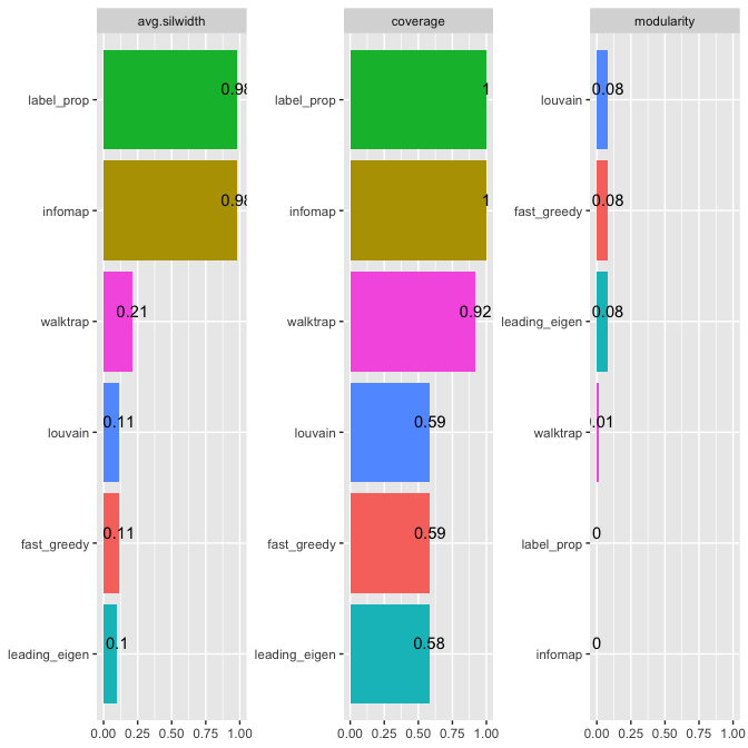
The predictEdge() function predicts new edges between
nominal variables’ labels or imputes missing values in the input data
matrix using several imputation methods. We can compare the imputation
results using the validateEdgePrediction() function to
choose the best method based on a predefined benchmark. The package
vignette and help manual contain more details.
imputations <- predictEdge(
  inc_mat = beatAML_incidence_matrix,
  method = c('svd','median','als','CA')
)validateEdgePrediction(imputation = imputations,
refer_community = cls$fast_greedy,
clustering_args = cls$clustering_args)
#>
#>
#> | | Jaccard_similarity| Dice_similarity_coefficient| Rand_index| Minkowski (inversed)| Fowlkes_Mallows_index|
#> |:------|------------------:|---------------------------:|----------:|--------------------:|---------------------:|
#> |median | 0.7476353| 0.8555964| 0.8628983| 1.870228| 0.8556407|
#> |svd | 0.7224792| 0.8388829| 0.8458376| 1.763708| 0.8388853|
#> |als | 0.7599244| 0.8635875| 0.8694758| 1.916772| 0.8635900|
#> |CA | 0.6935897| 0.8190765| 0.8280576| 1.670030| 0.8191111|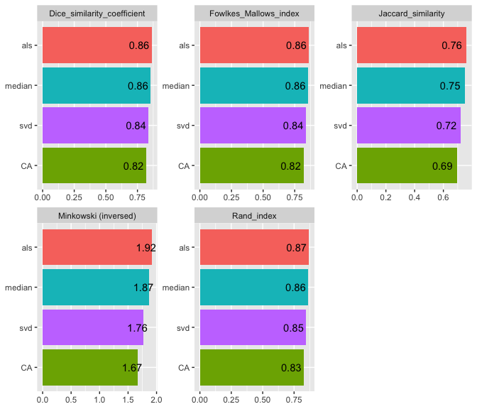
#>   imputation_method Jaccard_similarity Dice_similarity_coefficient Rand_index
#> 1            median          0.7476353                   0.8555964  0.8628983
#> 2               svd          0.7224792                   0.8388829  0.8458376
#> 3               als          0.7599244                   0.8635875  0.8694758
#> 4                CA          0.6935897                   0.8190765  0.8280576
#>   Minkowski (inversed) Fowlkes_Mallows_index
#> 1             1.870228             0.8556407
#> 2             1.763708             0.8388853
#> 3             1.916772             0.8635900
#> 4 1.670030 0.8191111![]()