![]()
<a href="https://CRAN.R-project.org/package=GPCERF">
    <img src="https://www.r-pkg.org/badges/version-last-release/GPCERF" alt="CRAN Package Version">
</a>
<a href="https://joss.theoj.org/papers/10.21105/joss.05465">
    <img src="https://joss.theoj.org/papers/10.21105/joss.05465/status.svg" alt="JOSS Status">
</a>
<a href="https://github.com/NSAPH-Software/GPCERF/actions">
    <img src="https://github.com/NSAPH-Software/GPCERF/workflows/R-CMD-check/badge.svg", alt="R-CMD-check status">
</a>
<a href="https://app.codecov.io/gh/NSAPH-Software/GPCERF">
    <img src="https://codecov.io/gh/NSAPH-Software/GPCERF/branch/develop/graph/badge.svg?token=066ISL822N", alt="Codecov">
</a>
<a href="http://www.r-pkg.org/pkg/GPCERF">
    <img src="https://cranlogs.r-pkg.org/badges/grand-total/GPCERF" alt="CRAN RStudio Mirror Downloads">
</a>
Gaussian Process (GP) and nearest neighbor Gaussian Process (nnGP) approaches for nonparametric modeling.
library("devtools")
install_github("NSAPH-Software/GPCERF", ref="develop")
library("GPCERF")Note: The following examples will also need installing
ranger R package.
library(GPCERF)
set.seed(781)
sim_data <- generate_synthetic_data(sample_size = 500, gps_spec = 1)
n_core <- 1
m_xgboost <- function(nthread = n_core, ...) {
SuperLearner::SL.xgboost(nthread = nthread, ...)
}
m_ranger <- function(num.threads = n_core, ...){
SuperLearner::SL.ranger(num.threads = num.threads, ...)
}
# Estimate GPS function
gps_m <- estimate_gps(cov_mt = sim_data[,-(1:2)],
w_all = sim_data$treat,
sl_lib = c("m_xgboost", "m_ranger"),
dnorm_log = TRUE)
# exposure values
q1 <- stats::quantile(sim_data$treat, 0.05)
q2 <- stats::quantile(sim_data$treat, 0.95)
w_all <- seq(q1, q2, 1)
params_lst <- list(alpha = 10 ^ seq(-2, 2, length.out = 10),
beta = 10 ^ seq(-2, 2, length.out = 10),
g_sigma = c(0.1, 1, 10),
tune_app = "all")
cerf_gp_obj <- estimate_cerf_gp(sim_data,
w_all,
gps_m,
params = params_lst,
outcome_col = "Y",
treatment_col = "treat",
covariates_col = paste0("cf", seq(1,6)),
nthread = n_core)
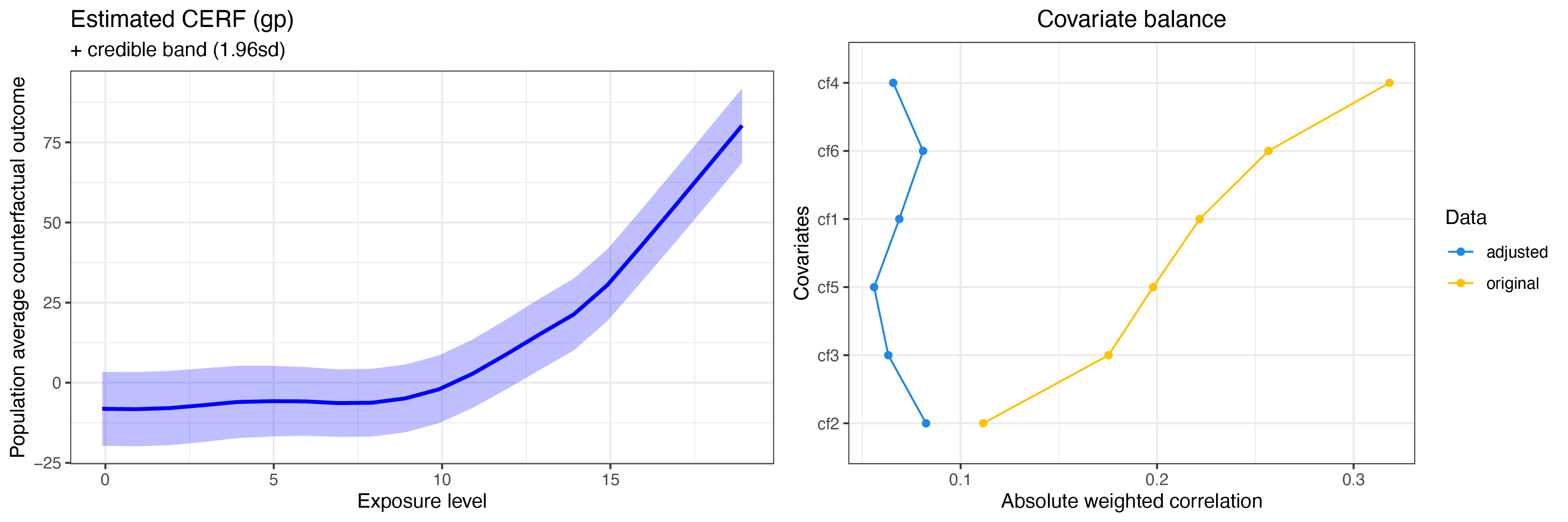
summary(cerf_gp_obj)
plot(cerf_gp_obj)GPCERF standard Gaussian grocess exposure response function object
Optimal hyper parameters(#trial: 300):
alpha = 12.9154966501488 beta = 12.9154966501488 g_sigma = 0.1
Optimal covariate balance:
cf1 = 0.069
cf2 = 0.082
cf3 = 0.063
cf4 = 0.066
cf5 = 0.056
cf6 = 0.081
Original covariate balance:
cf1 = 0.222
cf2 = 0.112
cf3 = 0.175
cf4 = 0.318
cf5 = 0.198
cf6 = 0.257
----***----
set.seed(781)
sim_data <- generate_synthetic_data(sample_size = 5000, gps_spec = 1)
m_xgboost <- function(nthread = 12, ...) {
SuperLearner::SL.xgboost(nthread = nthread, ...)
}
m_ranger <- function(num.threads = 12, ...){
SuperLearner::SL.ranger(num.threads = num.threads, ...)
}
# Estimate GPS function
gps_m <- estimate_gps(cov_mt = sim_data[,-(1:2)],
w_all = sim_data$treat,
sl_lib = c("m_xgboost", "m_ranger"),
dnorm_log = TRUE)
# exposure values
q1 <- stats::quantile(sim_data$treat, 0.05)
q2 <- stats::quantile(sim_data$treat, 0.95)
w_all <- seq(q1, q2, 1)
params_lst <- list(alpha = 10 ^ seq(-2, 2, length.out = 10),
beta = 10 ^ seq(-2, 2, length.out = 10),
g_sigma = c(0.1, 1, 10),
tune_app = "all",
n_neighbor = 50,
block_size = 1e3)
cerf_nngp_obj <- estimate_cerf_nngp(sim_data,
w_all,
gps_m,
params = params_lst,
outcome_col = "Y",
treatment_col = "treat",
covariates_col = paste0("cf", seq(1,6)),
nthread = 12)
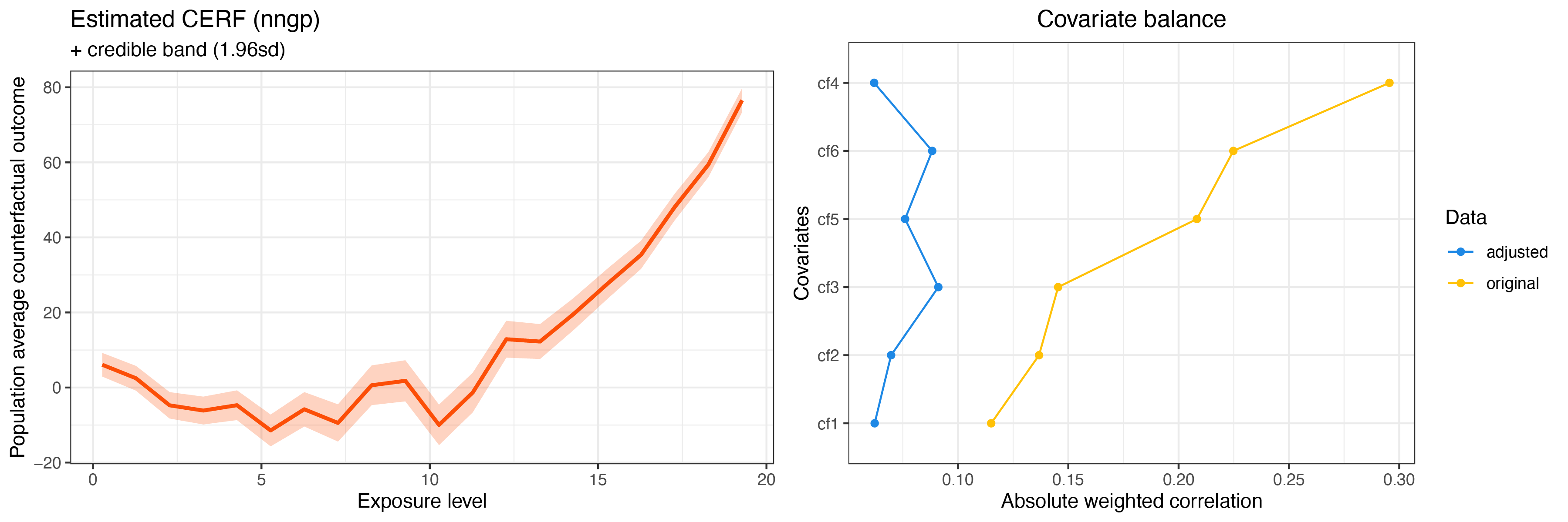
summary(cerf_nngp_obj)
plot(cerf_nngp_obj)GPCERF nearest neighbore Gaussian process exposure response function object summary
Optimal hyper parameters(#trial: 300):
alpha = 0.0278255940220712 beta = 0.215443469003188 g_sigma = 0.1
Optimal covariate balance:
cf1 = 0.062
cf2 = 0.070
cf3 = 0.091
cf4 = 0.062
cf5 = 0.076
cf6 = 0.088
Original covariate balance:
cf1 = 0.115
cf2 = 0.137
cf3 = 0.145
cf4 = 0.296
cf5 = 0.208
cf6 = 0.225
----***----
Please note that the GPCERF project is released with a Contributor Code of Conduct. By contributing to this project, you agree to abide by its terms.
Contributions to the package are encouraged. For detailed information on how to contribute, please refer to the CONTRIBUTING guidelines.
If you encounter any issues with GPCERF, we kindly ask you to report them on our GitHub by opening a new issue. To expedite resolution, including a reproducible example is highly appreciated. For those seeking assistance or further details about a particular topic, feel free to initiate a Discussion on GitHub or open an issue. Additionally, for more direct inquiries, the package maintainer can be reached via the email address provided in the DESCRIPTION file.
Ren, B., Wu, X., Braun, D., Pillai, N. and Dominici, F., 2021. Bayesian modeling for exposure response curve via gaussian processes: Causal effects of exposure to air pollution on health outcomes. arXiv preprint doi:10.48550/arXiv.2105.03454.