![]()
![]()
This is an R package that provides simple functions for creating contour plots.
The main functions are:
cf_grid: Makes a contour plot from grid
data.
cf_func: Makes a contour plot for a
function.
cf_data: Makes a contour plot for a data set by
fitting a Gaussian process model.
cf: Passes arguments to cf_function or
cf_data depending on whether the first argument is a
function or numeric.
All of these functions make the plot using base graphics by default.
To make plots using ggplot2, add the argument gg=TRUE, or
put g in front of the function name. E.g., gcf_data(...) is
the same as cf_data(..., gg=TRUE), and makes a similar plot
to cf_data but using ggplot2.
There are two functions for making plots in higher dimensions:
cf_4dim: Plots functions with four inputs by making
a series of contour plots.
cf_highdim: Plots for higher dimensional inputs by
making a contour plot for each pair of input dimensions and holding the
other inputs constant or averaging over them.
# It can be installed like any other package
install.packages("ContourFunctions")

# Or the the development version from GitHub:
# install.packages("devtools")
devtools::install_github("CollinErickson/contour")Plot a grid of data:
library(ContourFunctions)
a <- b <- seq(-4*pi, 4*pi, len = 27)
r <- sqrt(outer(a^2, b^2, "+"))
cf_grid(a, b, cos(r^2)*exp(-r/(2*pi)))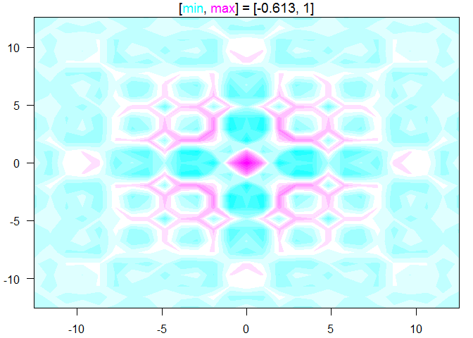
Plot a function with two input dimensions:
f1 <- function(r) cos(r[1]^2 + r[2]^2)*exp(-sqrt(r[1]^2 + r[2]^2)/(2*pi))
cf_func(f1, xlim = c(-4*pi, 4*pi), ylim = c(-4*pi, 4*pi))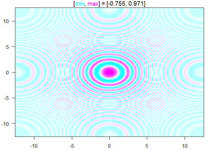
Using data with two inputs and an output, fit a Gaussian process model and show the contour surface with dots where the points are:
set.seed(0)
x <- runif(20)
y <- runif(20)
z <- exp(-(x-.5)^2-5*(y-.5)^2)
cf_data(x,y,z)
#> Fitting with laGP since n <= 200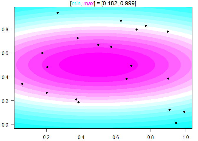
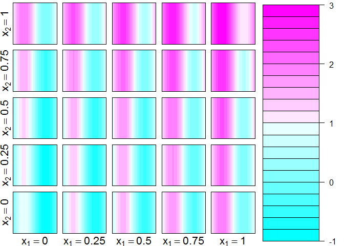
For more than two input dimensions:
friedman <- function(x) {
  10*sin(pi*x[1]*x[2]) + 20*(x[3]-.5)^2 + 10*x[4] + 5*x[5]
}
cf_highdim(friedman, 5, color.palette=topo.colors)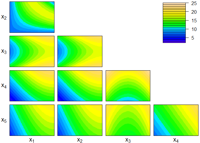
For (three or) four inputs dimensions:
cf_4dim(function(x) {x[1] + x[2]^2 + sin(2*pi*x[3])})