![]()
![]()
ARDL creates complex autoregressive distributed lag
(ARDL) models and constructs the underlying unrestricted and restricted
error correction model (ECM) automatically, just by providing the order.
It also performs the bounds-test for cointegration as described in Pesaran
et al. (2001) and provides the multipliers and the cointegrating
equation. The validity and the accuracy of this package have been
verified by successfully replicating the results of Pesaran et
al. (2001) in Natsiopoulos
and Tzeremes (2022).
ARDL?# You can install the released version of ARDL from CRAN:
install.packages("ARDL")
# Or the latest development version from GitHub:
install.packages("devtools")
devtools::install_github("Natsiopoulos/ARDL")This is a basic example which shows how to use the main functions of
the ARDL package.
Assume that we want to model the LRM (logarithm of real
money, M2) as a function of LRY, IBO and
IDE (see ?denmark). The problem is that
applying an OLS regression on non-stationary data would result into a
spurious regression. The estimated parameters would be consistent only
if the series were cointegrated.
library(ARDL)
data(denmark)
First, we find the best ARDL specification. We search up to order 5.
models <- auto_ardl(LRM ~ LRY + IBO + IDE, data = denmark, max_order = 5)

# The top 20 models according to the AIC
models$top_orders
#>    LRM LRY IBO IDE       AIC
#> 1    3   1   3   2 -251.0259
#> 2    3   1   3   3 -250.1144
#> 3    2   2   0   0 -249.6266
#> 4    3   2   3   2 -249.1087
#> 5    3   2   3   3 -248.1858
#> 6    2   2   0   1 -247.7786
#> 7    2   1   0   0 -247.5643
#> 8    2   2   1   1 -246.6885
#> 9    3   3   3   3 -246.3061
#> 10   2   2   1   2 -246.2709
#> 11   2   1   1   1 -245.8736
#> 12   2   2   2   2 -245.7722
#> 13   1   1   0   0 -245.6620
#> 14   2   1   2   2 -245.1712
#> 15   3   1   2   2 -245.0996
#> 16   1   0   0   0 -244.4317
#> 17   1   1   0   1 -243.7702
#> 18   5   5   5   5 -243.3120
#> 19   4   1   3   2 -243.0728
#> 20   4   1   3   3 -242.4378

# The best model was found to be the ARDL(3,1,3,2)
ardl_3132 <- models$best_model
ardl_3132$order
#> LRM LRY IBO IDE
#>   3   1   3   2
summary(ardl_3132)
#>
#> Time series regression with "zooreg" data:
#> Start = 1974 Q4, End = 1987 Q3
#>
#> Call:
#> dynlm::dynlm(formula = full_formula, data = data, start = start,
#>     end = end)
#>
#> Residuals:
#>       Min        1Q    Median        3Q       Max
#> -0.029939 -0.008856 -0.002562  0.008190  0.072577
#>
#> Coefficients:
#>             Estimate Std. Error t value Pr(>|t|)
#> (Intercept)   2.6202     0.5678   4.615 4.19e-05 ***
#> L(LRM, 1)     0.3192     0.1367   2.336 0.024735 *
#> L(LRM, 2)     0.5326     0.1324   4.024 0.000255 ***
#> L(LRM, 3)    -0.2687     0.1021  -2.631 0.012143 *
#> LRY           0.6728     0.1312   5.129 8.32e-06 ***
#> L(LRY, 1)    -0.2574     0.1472  -1.749 0.088146 .
#> IBO          -1.0785     0.3217  -3.353 0.001790 **
#> L(IBO, 1)    -0.1062     0.5858  -0.181 0.857081
#> L(IBO, 2)     0.2877     0.5691   0.505 0.616067
#> L(IBO, 3)    -0.9947     0.3925  -2.534 0.015401 *
#> IDE           0.1255     0.5545   0.226 0.822161
#> L(IDE, 1)    -0.3280     0.7213  -0.455 0.651847
#> L(IDE, 2)     1.4079     0.5520   2.550 0.014803 *
#> ---
#> Signif. codes:  0 '***' 0.001 '**' 0.01 '*' 0.05 '.' 0.1 ' ' 1
#>
#> Residual standard error: 0.0191 on 39 degrees of freedom
#> Multiple R-squared:  0.988,  Adjusted R-squared:  0.9843
#> F-statistic: 266.8 on 12 and 39 DF,  p-value: < 2.2e-16
Then we can estimate the UECM (Unrestricted Error Correction Model) of the underlying ARDL(3,1,3,2).
uecm_3132 <- uecm(ardl_3132)
summary(uecm_3132)
#>
#> Time series regression with "zooreg" data:
#> Start = 1974 Q4, End = 1987 Q3
#>
#> Call:
#> dynlm::dynlm(formula = full_formula, data = data, start = start,
#>     end = end)
#>
#> Residuals:
#>       Min        1Q    Median        3Q       Max
#> -0.029939 -0.008856 -0.002562  0.008190  0.072577
#>
#> Coefficients:
#>              Estimate Std. Error t value Pr(>|t|)
#> (Intercept)   2.62019    0.56777   4.615 4.19e-05 ***
#> L(LRM, 1)    -0.41685    0.09166  -4.548 5.15e-05 ***
#> L(LRY, 1)     0.41538    0.11761   3.532  0.00108 **
#> L(IBO, 1)    -1.89172    0.39111  -4.837 2.09e-05 ***
#> L(IDE, 1)     1.20534    0.44690   2.697  0.01028 *
#> d(L(LRM, 1)) -0.26394    0.10192  -2.590  0.01343 *
#> d(L(LRM, 2))  0.26867    0.10213   2.631  0.01214 *
#> d(LRY)        0.67280    0.13116   5.129 8.32e-06 ***
#> d(IBO)       -1.07852    0.32170  -3.353  0.00179 **
#> d(L(IBO, 1))  0.70701    0.46874   1.508  0.13953
#> d(L(IBO, 2))  0.99468    0.39251   2.534  0.01540 *
#> d(IDE)        0.12546    0.55445   0.226  0.82216
#> d(L(IDE, 1)) -1.40786    0.55204  -2.550  0.01480 *
#> ---
#> Signif. codes:  0 '***' 0.001 '**' 0.01 '*' 0.05 '.' 0.1 ' ' 1
#>
#> Residual standard error: 0.0191 on 39 degrees of freedom
#> Multiple R-squared:  0.7458, Adjusted R-squared:  0.6676
#> F-statistic: 9.537 on 12 and 39 DF,  p-value: 3.001e-08
And also the RECM (Restricted Error Correction Model) of the underlying ARDL(3,1,3,2), allowing the constant to join the long-run relationship (case 2), instead of the short-run (case 3).
recm_3132 <- recm(uecm_3132, case = 2)
summary(recm_3132)
#>
#> Time series regression with "zooreg" data:
#> Start = 1974 Q4, End = 1987 Q3
#>
#> Call:
#> dynlm::dynlm(formula = full_formula, data = data, start = start,
#>     end = end)
#>
#> Residuals:
#>       Min        1Q    Median        3Q       Max
#> -0.029939 -0.008856 -0.002562  0.008190  0.072577
#>
#> Coefficients:
#>              Estimate Std. Error t value Pr(>|t|)
#> d(L(LRM, 1)) -0.26394    0.09008  -2.930 0.005405 **
#> d(L(LRM, 2))  0.26867    0.09127   2.944 0.005214 **
#> d(LRY)        0.67280    0.11591   5.805 7.03e-07 ***
#> d(IBO)       -1.07852    0.30025  -3.592 0.000837 ***
#> d(L(IBO, 1))  0.70701    0.44359   1.594 0.118300
#> d(L(IBO, 2))  0.99468    0.36491   2.726 0.009242 **
#> d(IDE)        0.12546    0.48290   0.260 0.796248
#> d(L(IDE, 1)) -1.40786    0.48867  -2.881 0.006160 **
#> ect          -0.41685    0.07849  -5.311 3.63e-06 ***
#> ---
#> Signif. codes:  0 '***' 0.001 '**' 0.01 '*' 0.05 '.' 0.1 ' ' 1
#>
#> Residual standard error: 0.01819 on 43 degrees of freedom
#>   (0 observations deleted due to missingness)
#> Multiple R-squared:  0.7613, Adjusted R-squared:  0.7113
#> F-statistic: 15.24 on 9 and 43 DF,  p-value: 9.545e-11
Let’s test if there is a long-run levels relationship (cointegration) using the bounds test from Pesaran et al. (2001).
# The bounds F-test (under the case 2) rejects the NULL hypothesis (let's say, assuming alpha = 0.01) with p-value = 0.004418.
bounds_f_test(ardl_3132, case = 2)
#>
#>  Bounds F-test (Wald) for no cointegration
#>
#> data:  d(LRM) ~ L(LRM, 1) + L(LRY, 1) + L(IBO, 1) + L(IDE, 1) + d(L(LRM,     1)) + d(L(LRM, 2)) + d(LRY) + d(IBO) + d(L(IBO, 1)) + d(L(IBO,     2)) + d(IDE) + d(L(IDE, 1))
#> F = 5.1168, p-value = 0.004418
#> alternative hypothesis: Possible cointegration
#> null values:
#>    k    T
#>    3 1000

# The bounds t-test (under the case 3) rejects the NULL hypothesis (let's say, assuming alpha = 0.01) with p-value = 0.005538.
# We also provide the critical value bounds for alpha = 0.01.
tbounds <- bounds_t_test(uecm_3132, case = 3, alpha = 0.01)
tbounds
#>
#>  Bounds t-test for no cointegration
#>
#> data:  d(LRM) ~ L(LRM, 1) + L(LRY, 1) + L(IBO, 1) + L(IDE, 1) + d(L(LRM,     1)) + d(L(LRM, 2)) + d(LRY) + d(IBO) + d(L(IBO, 1)) + d(L(IBO,     2)) + d(IDE) + d(L(IDE, 1))
#> t = -4.5479, Lower-bound I(0) = -3.4430, Upper-bound I(1) = -4.3799,
#> p-value = 0.005538
#> alternative hypothesis: Possible cointegration
#> null values:
#>    k    T
#>    3 1000

# Here is a more clear view of the main results.
tbounds$tab
#>   statistic Lower-bound I(0) Upper-bound I(1) alpha     p.value
#> t -4.547939        -3.442978        -4.379886  0.01 0.005538316
Here we have the short-run and the long-run multipliers (with standard errors, t-statistics and p-values).
multipliers(ardl_3132, type = "sr")
#>          Term   Estimate Std. Error    t value     Pr(>|t|)
#> 1 (Intercept)  2.6201916  0.5677679  4.6148990 4.186867e-05
#> 2         LRY  0.6727993  0.1311638  5.1294603 8.317401e-06
#> 3         IBO -1.0785180  0.3217011 -3.3525465 1.790030e-03
#> 4         IDE  0.1254643  0.5544522  0.2262852 8.221614e-01
multipliers(ardl_3132)
#>          Term   Estimate Std. Error   t value     Pr(>|t|)
#> 1 (Intercept)  6.2856579  0.7719160  8.142930 6.107445e-10
#> 2         LRY  0.9964676  0.1239310  8.040503 8.358472e-10
#> 3         IBO -4.5381160  0.5202961 -8.722180 1.058619e-10
#> 4         IDE  2.8915201  0.9950853  2.905801 6.009239e-03
We can also estimate and visualize the delay multipliers along with their standard errors.
mult15 <- multipliers(ardl_3132, type = 15, se = TRUE)
plot_delay(mult15, interval = 0.95)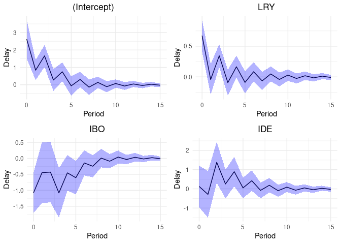
Now let’s graphically check the estimated long-run relationship
(cointegrating equation) against the dependent variable
LRM.
ce <- coint_eq(ardl_3132, case = 2)plot_lr(ardl_3132, coint_eq = ce, show.legend = TRUE)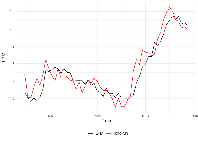
Forecasting and using an ardl, uecm, or
recm model in other functions are easy as they can be
converted in regular lm models.
ardl_3132_lm <- to_lm(ardl_3132)

# Forecast using the in-sample data
insample_data <- ardl_3132$model
predicted_values <- predict(ardl_3132_lm, newdata = insample_data)

# Convert to ts class for the plot
predicted_values <- ts(predicted_values, start = c(1974,4), frequency=4)
plot(denmark$LRM, lwd=2) #The input dependent variable
lines(predicted_values, col="red", lwd=2) #The predicted values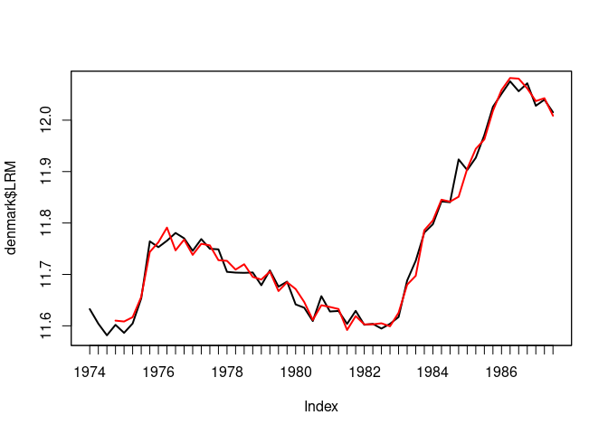
Let’s see what it takes to build the above ARDL(3,1,3,2) model.
Using the ARDL package (literally one line of
code):
ardl_model <- ardl(LRM ~ LRY + IBO + IDE, data = denmark, order = c(3,1,3,2))Without the ARDL package:
(Using the dynlm package, because striving with the
lm function would require extra data transformation to
behave like time-series)
library(dynlm)
#> Loading required package: zoo
#>
#> Attaching package: 'zoo'
#> The following objects are masked from 'package:base':
#>
#>     as.Date, as.Date.numeric

dynlm_ardl_model <- dynlm(LRM ~ L(LRM, 1) + L(LRM, 2) + L(LRM, 3) + LRY + L(LRY, 1) +
                           IBO + L(IBO, 1) + L(IBO, 2) + L(IBO, 3) +
IDE + L(IDE, 1) + L(IDE, 2), data = denmark)identical(ardl_model$coefficients, dynlm_ardl_model$coefficients)
#> [1] TRUEAn ARDL model has a relatively simple structure, although the difference in typing effort is noticeable.
Not to mention the complex transformation for an ECM. The extra typing is the least of your problems trying to do this. First you would need to figure out the exact structure of the model!
Using the ARDL package (literally one line of
code):
uecm_model <- uecm(ardl_model)Without the ARDL package:
dynlm_uecm_model <- dynlm(d(LRM) ~ L(LRM, 1) + L(LRY, 1) + L(IBO, 1) +
                                   L(IDE, 1) + d(L(LRM, 1)) + d(L(LRM, 2)) +
                                   d(LRY) + d(IBO) + d(L(IBO, 1)) + d(L(IBO, 2)) +
d(IDE) + d(L(IDE, 1)), data = denmark)identical(uecm_model$coefficients, dynlm_uecm_model$coefficients)
#> [1] TRUENatsiopoulos, Kleanthis, & Tzeremes, Nickolaos G. (2022). ARDL bounds test for cointegration: Replicating the Pesaran et al. (2001) results for the UK earnings equation using R. Journal of Applied Econometrics, 37(5), 1079-1090. https://doi.org/10.1002/jae.2919
Pesaran, M. H., Shin, Y., & Smith, R. J. (2001). Bounds testing approaches to the analysis of level relationships. Journal of Applied Econometrics, 16(3), 289-326